Lab 11: Multitype summary functions and models

This session is concerned with summary statistics and Gibbs models for multitype point patterns. The lecturer’s R script is available here (right click and save).

library(spatstat)

Exercise 1

The amacrine dataset contains the locations of cells of two types (“on” and “off” detectors) in a layer of the retina.

Compute and plot the bivariate L function for the amacrine data.
```
Lam <- alltypes(amacrine, "L")
plot(Lam)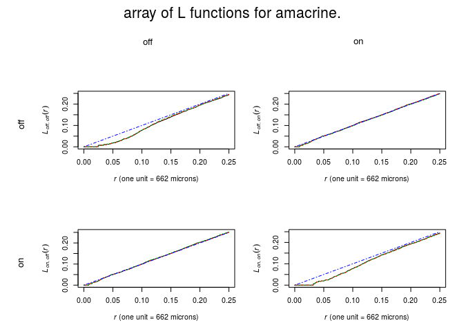
```
plot estimates of the bivariate pair correlation functions by
```
plot(alltypes(amacrine, pcfcross))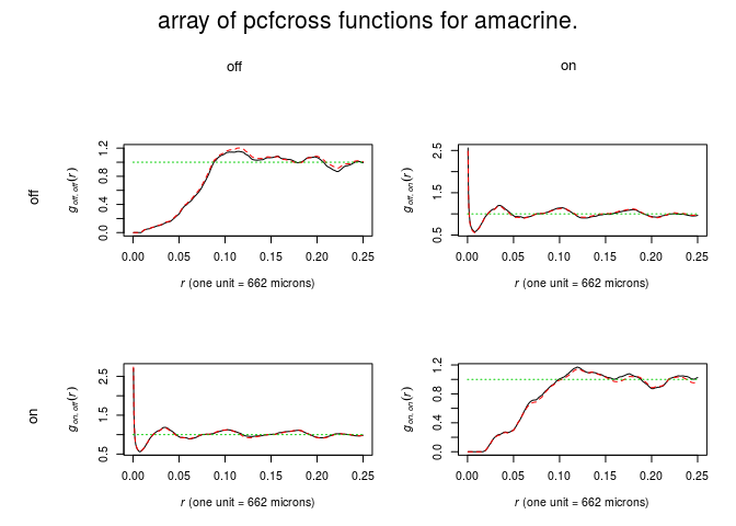
```
What is the overall interpretation of these summary functions?

Inhibition for types of same type. Independence between types.

Exercise 2

Continuing with the amacrine data,

Use alltypes to plot the bivariate G-functions G_i**j for each pair of types i, j in the amacrine data.
```
plot(alltypes(amacrine, Gcross))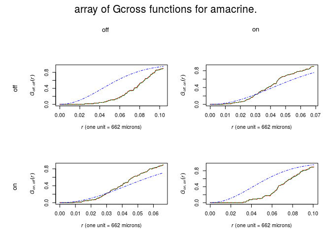
```
Use alltypes to plot the functions G_i• (Gdot in spatstat) for each type i in the amacrine data.
```
plot(alltypes(amacrine, Gdot))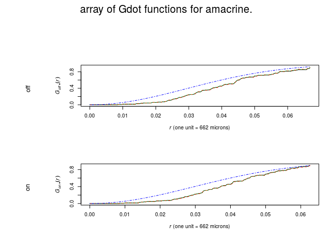
```
What is the overall interpretation of the G-functions?

Same as before.

Exercise 3

The dataset bramblecanes gives the locations and ages of bramble cane plants in a study region. Age is a categorical variable, with three levels. We will conduct a randomisation test of the Random Labelling Property.

Read the help for the command rlabel.
We will use the bivariate K-function K_2, 0 as our summary statistic. Compute this for the data using Kcross(bramblecanes, "2", "0") and plot it.
```
plot(Kcross(bramblecanes, "2", "0"))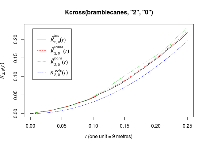
```
Read the help for Kcross. Find the names of the second and third arguments to the function.

The names are i and j. Alternatively the arguments from and to can be used for the same purpose.

Generate the simulation envelopes as follows

shuffle <- expression(rlabel(bramblecanes))
E <- envelope(bramblecanes, Kcross, nsim=19, simulate=shuffle, i="2", j="0")

## Generating 19 simulations by evaluating expression  ...
## 1, 2, 3, 4, 5, 6, 7, 8, 9, 10, 11, 12, 13, 14, 15, 16, 17, 18,  19.
## 
## Done.

plot(E)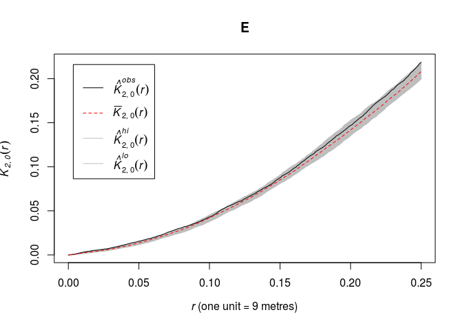

Note that the named arguments i and j are not recognised by the envelope command (as we can check from the help file for envelope), so they are passed to the command Kcross as we intended.

Generate the corresponding simulation envelopes of the bivariate L-function, either by replacing Kcross by Lcross in the code above, or by
```
plot(E, sqrt(./pi) ~ r)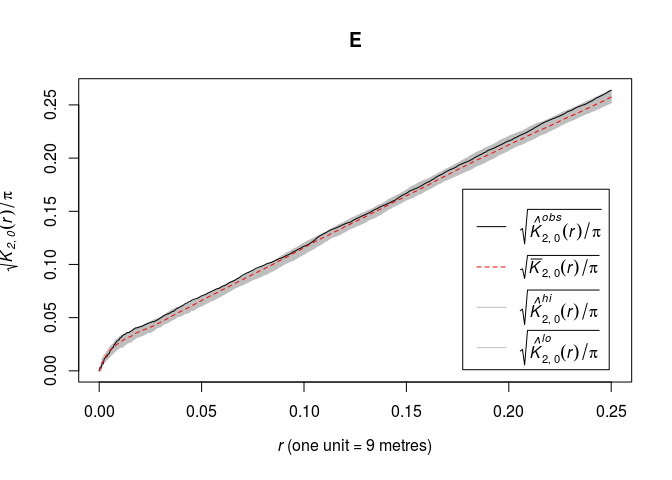
```

Exercise 4

We want to fit a Gibbs process model to the betacells data.

Access the betacells data and plot the pattern.
```
plot(betacells, main = "Beta cells")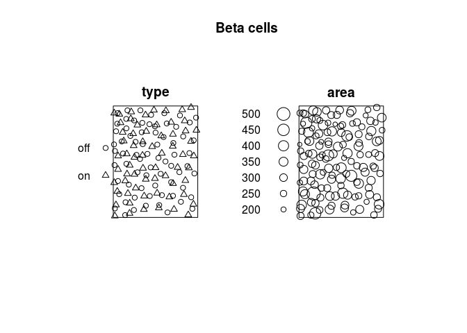
```
Save the data as a point pattern X and save only the mark type
```
X <- betacells
marks(X) <- marks(betacells)$type
```
Also we will save the two type names:
```
typ <- levels(marks(X))
```
Plot the bivariate K functions.
1. Does it appear that cells of the same type interact? If so, guess at a suitable interaction distance.
2. Does it appear that cells of different types interact? If so, guess at a suitable interaction distance.
```
plot(alltypes(X, Kcross))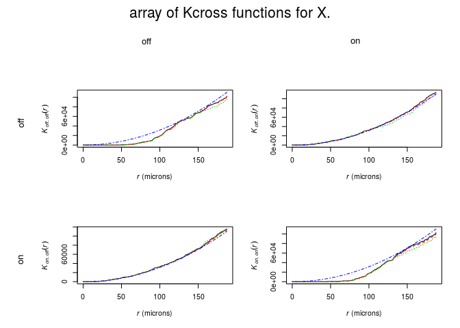
```
Yes, points of same type appear to be interacting at e.g. 60 microns.

No, points of opposite types do not appear to interact (or if they do it is only at quite short distances).
Fit a multitype Strauss model using the selected interactions. For example if your answer to question i was “yes, at 20 microns” and your answer to question ii was “yes, at 30 microns”,
```
rad <- matrix(c(20,30,30,20), 2, 2)
ppm(X ~ marks, MultiStrauss(typ,rad))
```
while if your answer to question i was “no” and your answer to question ii was “yes, at 60 microns”,
```
rad <- matrix(c(NA,60,60,NA), 2, 2)
ppm(X ~ marks, MultiStrauss(typ,rad))
```
```
rad <- matrix(c(60,NA,NA,60), 2, 2)
fit <- ppm(X ~ marks, MultiStrauss(typ,rad))
```
Interpret the fitted model. Plot the array of fitted pairwise interactions using plot(fitin(fit)) where fit is the fitted model. What is the fitted strength of the interaction?
```
plot(fitin(fit))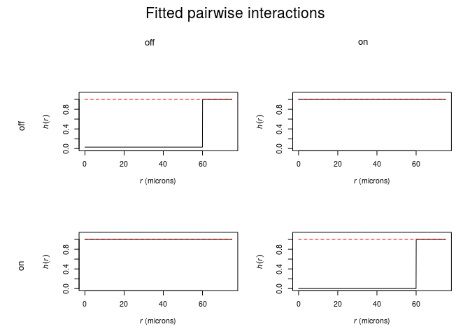
```
The fitted interaction is very strong for same type cells (and absent for opposite types).

For comparison purposes, fit the following models, interpret them, and compare the results:

fitU <- ppm(X ~ marks, Strauss(60))
rad <- matrix(60, 2, 2)
fitE <- ppm(X ~ marks, MultiStrauss(rad))

Exercise 5

Here we will use profile pseudolikelihood to estimate the interaction distances for the multitype Strauss model in Question 4. We’ll assume that points of different types do not interact, and that points of the same type interact at a distance R which is the same for each type.

Create a vector of values of R to search over:
```
rval <- data.frame(R=seq(50,100,by=5))
```
This will become the argument s of profilepl.

We need the argument f of profilepl, and this should be a function that takes the value R and produces a multitype Strauss interaction. So define

MS <- function(R){ MultiStrauss(diag(c(R,R))) }

Try typing MS(50) to check that this is what you expect.

MS(50)

## Pairwise interaction family
## Interaction:Multitype Strauss process
## 2 types of points
## Possible types:   not yet determined
## Interaction radii:
##      [,1] [,2]
## [1,]   50   NA
## [2,]   NA   50

Then we can use maximum profile pseudolikelihood:

profilepl(rval, MS, X ~ marks)

## (computing rbord)

## comparing 11 models...

## 1, 2, 3, 4, 5, 6, 7, 8, 9, 10,  11.

## fitting optimal model...

## done.

## profile log pseudolikelihood
## for model:  ppm(X ~ marks,  interaction = MS)
## fitted with rbord = 100
## interaction: Multitype Strauss process
## irregular parameter: R in [50, 100]
## optimum value of irregular parameter:  R = 80