Lab 10: Gibbs processes
This session is concerned with Gibbs models for point patterns with interpoint interaction. The lecturer’s R script is available here (right click and save).
library(spatstat)
Exercise 1
In this question we fit a Strauss point process model to the swedishpines data.
-
We need a guess at the interaction distance R. Compute and plot the L-function of the dataset and choose the value r which maximises the discrepancy L(r)−r . We plot the above function which we want to maximize.
plot(Lest(swedishpines), abs(iso - r) ~ r, main = "")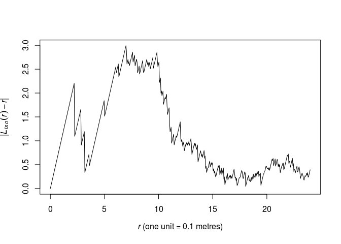
As seen from the plot, the maximum lies around r = 6.5 by eye. We find the optimum explicitly like follows:
discrep <- function(r) {
  return(abs(as.function(Lest(swedishpines))(r) - r))
}
res <- optimise(discrep, interval = c(0.1, 20), maximum = TRUE)
print(res)
## $maximum ## [1] 6.984333 ## ## $objective ## [1] 2.992058R <- res$maximumThis corresponds nicely with the plot.
-
Fit the stationary Strauss model with the chosen interaction distance using
ppm(swedishpines ~ 1, Strauss(R))where
Ris your chosen value. -
Interpret the printout: how strong is the interaction?
-
Plot the fitted pairwise interaction function using
plot(fitin(fit)).As we have assigned
R, we simply write:fit <- ppm(swedishpines ~ 1, Strauss(R)) print(fit)## Stationary Strauss process ## ## First order term: beta = 0.0281221 ## ## Interaction distance: 6.984333 ## Fitted interaction parameter gamma: 0.1434456 ## ## Relevant coefficients: ## Interaction ## -1.941799 ## ## For standard errors, type coef(summary(x))As seen, the γ = 0.14 parameter is quite small. Thus there seems to be a strong negative association between points within distance R of each other. A γ of 0 implies the hard core process whereas γ = 1 implies the Poisson process and thus CSR.
The pairwise interaction function become:
plot(fitin(fit))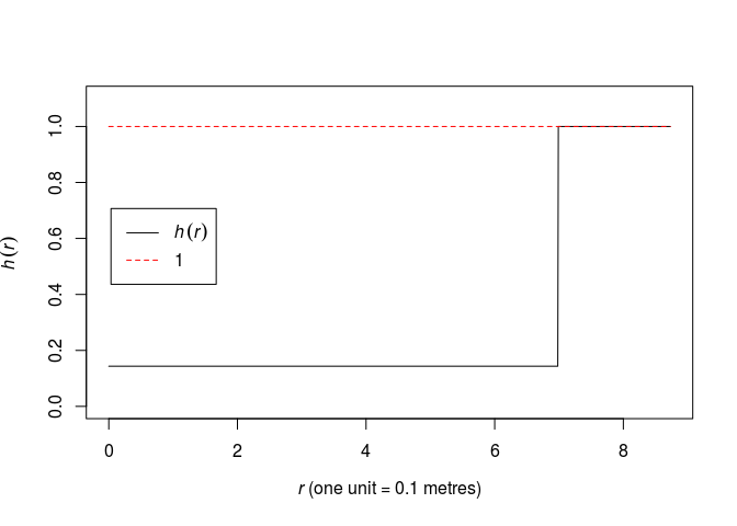
Exercise 2
In Question 1 we guesstimated the Strauss interaction distance parameter. Alternatively this parameter could be estimated by profile pseudolikelihood.
-
Look again at the plot of the L-function of
swedishpinesand determine a plausible range of possible values for the interaction distance.plot(Lest(swedishpines), main = "")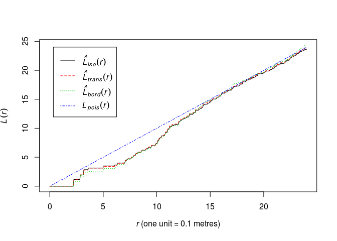
A conservative range of plausible interaction distances seems to be 3 to 15 meters.
-
Generate a sequence of values equally spaced across this range, for example, if your range of plausible values was [0.05, 0.3], then type
rvals <- seq(0.05, 0.3, by=0.01)We generate the numbers between 3 and 12.
rvals <- seq(3, 12, by = 0.1) -
Construct a data frame, with one column named
r(matching the argument name ofStrauss), containing these values. For exampleD <- data.frame(r = rvals)OK,
D <- data.frame(r = rvals) -
Execute
fitp <- profilepl(D, Strauss, swedishpines ~ 1)to find the maximum profile pseudolikelihood fit.
OK, let’s execute it:
fitp <- profilepl(D, Strauss, swedishpines ~ 1)## (computing rbord) ## comparing 91 models... ## 1, 2, 3, 4, 5, 6, 7, 8, 9, 10, 11, 12, 13, 14, 15, 16, 17, 18, 19, 20, 21, 22, 23, 24, 25, 26, 27, 28, 29, 30, 31, 32, 33, 34, 35, 36, 37, 38, ## 39, 40, 41, 42, 43, 44, 45, 46, 47, 48, 49, 50, 51, 52, 53, 54, 55, 56, 57, 58, 59, 60, 61, 62, 63, 64, 65, 66, 67, 68, 69, 70, 71, 72, 73, 74, 75, 76, ## 77, 78, 79, 80, 81, 82, 83, 84, 85, 86, 87, 88, 89, 90, 91. ## fitting optimal model... ## done. -
Print and plot the object
fitp.print(fitp)## profile log pseudolikelihood ## for model: ppm(swedishpines ~ 1, interaction = Strauss) ## fitted with rbord = 12 ## interaction: Strauss process ## irregular parameter: r in [3, 12] ## optimum value of irregular parameter: r = 9.8plot(fitp)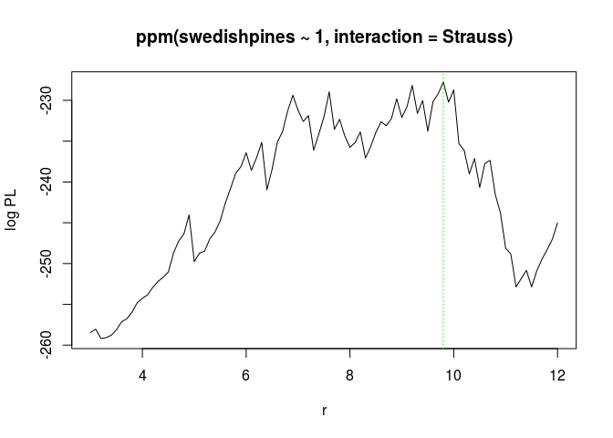
-
Compare the computed estimate of interaction distance r with your guesstimate. Compare the corresponding estimates of the Strauss interaction parameter γ.
(Ropt <- reach(as.ppm(fitp)))## [1] 9.8The r = 9.8 is not totally inconsistent with the previous estimate of 7.
-
Extract the fitted Gibbs point process model from the object
fitpasbestfit <- as.ppm(fitp)OK, let’s do that:
bestfit <- as.ppm(fitp)
Exercise 3
For the Strauss model fitted in Question 1,
-
Generate and plot a simulated realisation of the fitted model using
simulate.s <- simulate(fit, drop = TRUE) plot(s, main = "")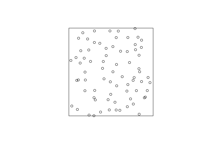
-
Plot the L-function of the data along with the global simulation envelopes from 19 realisations of the fitted model.
plot(envelope(fit, Lest, global = TRUE, nsim = 19, nsim2 = 100), main = "")## Generating 119 simulated realisations of fitted Gibbs model (100 to ## estimate the mean and 19 to calculate envelopes) ... ## 1, 2, 3, 4.6.8.10.12.14.16.18.20.22.24.26.28.30.32.34.36.38. ## 40.42.44.46.48.50.52.54.56.58.60.62.64.66.68.70.72.74.76.78 ## .80.82.84.86.88.90.92.94.96.98.100.102.104.106.108.110.112.114.116. ## 118 119. ## ## Done.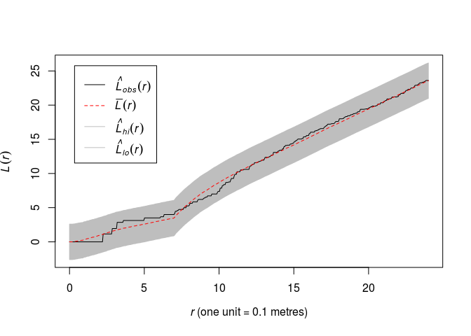
Exercise 4
-
Read the help file for
Geyer.See
help(Geyer) -
Fit a stationary Geyer saturation process to
swedishpines, with the same interaction distance as for the Strauss model computed in Question 2, and trying different values of the saturation parametersat = 1, 2, 3say.ppm(swedishpines ~ 1, Geyer(r = Ropt, sat = 1))## Stationary Geyer saturation process ## ## First order term: beta = 0.07472669 ## ## Interaction distance: 9.8 ## Saturation parameter: 1 ## Fitted interaction parameter gamma: 0.1871555 ## ## Relevant coefficients: ## Interaction ## -1.675815 ## ## For standard errors, type coef(summary(x))ppm(swedishpines ~ 1, Geyer(r = Ropt, sat = 2))## Stationary Geyer saturation process ## ## First order term: beta = 0.04707047 ## ## Interaction distance: 9.8 ## Saturation parameter: 2 ## Fitted interaction parameter gamma: 0.5242884 ## ## Relevant coefficients: ## Interaction ## -0.6457134 ## ## For standard errors, type coef(summary(x))ppm(swedishpines ~ 1, Geyer(r = Ropt, sat = 3))## Stationary Geyer saturation process ## ## First order term: beta = 0.07603509 ## ## Interaction distance: 9.8 ## Saturation parameter: 3 ## Fitted interaction parameter gamma: 0.5261429 ## ## Relevant coefficients: ## Interaction ## -0.6421823 ## ## For standard errors, type coef(summary(x)) -
Fit the same model with the addition of a log-quadratic trend.
gfit <- ppm(swedishpines ~ polynom(x, y, 2), Geyer(r = Ropt, sat = 3)) -
Plot the fitted trend and conditional intensity.
Here we use the log scale to be able to see the discs in the conditional intensity.
par(mfrow=c(1,2)) plot(gfit, log = TRUE, pause = FALSE)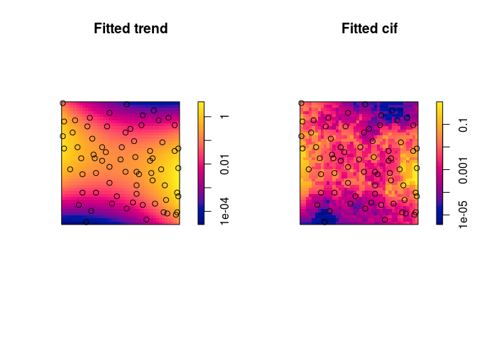
Exercise 5
Modify question 1 by using the Huang-Ogata approximate maximum likelihood algorithm (method="ho") instead of maximum pseudolikelihood (the default, method="mpl").
fit.mpl <- ppm(swedishpines ~ 1, Strauss(R), method = "mpl")
fit.ho <- ppm(swedishpines ~ 1, Strauss(R), method = "ho")
## Simulating... 1, 2, 3, 4, 5, 6, 7, 8, 9, 10, 11, 12, 13, 14, 15, 16, 17, 18, 19, 20, 21, 22, 23, 24, 25, 26, 27, 28, 29, 30, 31, 32, 33, 34, 35, 36, 37, 38,
## 39, 40, 41, 42, 43, 44, 45, 46, 47, 48, 49, 50, 51, 52, 53, 54, 55, 56, 57, 58, 59, 60, 61, 62, 63, 64, 65, 66, 67, 68, 69, 70, 71, 72, 73, 74, 75, 76,
## 77, 78, 79, 80, 81, 82, 83, 84, 85, 86, 87, 88, 89, 90, 91, 92, 93, 94, 95, 96, 97, 98, 99, 100.
## Done.
print(fit.ho)
## Stationary Strauss process
##
## First order term: beta = 0.03025998
##
## Interaction distance: 6.984333
## Fitted interaction parameter gamma: 0.1473619
##
## Relevant coefficients:
## Interaction
## -1.914864
##
## For standard errors, type coef(summary(x))
print(fit.mpl)
## Stationary Strauss process
##
## First order term:  beta = 0.0281221
##
## Interaction distance:    6.984333
## Fitted interaction parameter gamma:   0.1434456
##
## Relevant coefficients:
## Interaction
##   -1.941799
##
## For standard errors, type coef(summary(x))
The fits are very similar.
Exercise 6
Repeat Question 2 for the inhomogeneous Strauss process with log-quadratic trend. The corresponding call to profilepl is
fitp <- profilepl(D, Strauss, swedishpines ~ polynom(x,y,2))
fitp2 <- profilepl(D, Strauss, swedishpines ~ polynom(x,y,2))
## (computing rbord)

## comparing 91 models...

## 1, 2, 3, 4, 5, 6, 7, 8, 9, 10, 11, 12, 13, 14, 15, 16, 17, 18, 19, 20, 21, 22, 23, 24, 25, 26, 27, 28, 29, 30, 31, 32, 33, 34, 35, 36, 37, 38,
## 39, 40, 41, 42, 43, 44, 45, 46, 47, 48, 49, 50, 51, 52, 53, 54, 55, 56, 57, 58, 59, 60, 61, 62, 63, 64, 65, 66, 67, 68, 69, 70, 71, 72, 73, 74, 75, 76,
## 77, 78, 79, 80, 81, 82, 83, 84, 85, 86, 87, 88, 89, 90,  91.

## fitting optimal model...

## done.
print(fitp)
## profile log pseudolikelihood
## for model:  ppm(swedishpines ~ 1,  interaction = Strauss)
## fitted with rbord = 12
## interaction: Strauss process
## irregular parameter: r in [3, 12]
## optimum value of irregular parameter:  r = 9.8
print(fitp2)
## profile log pseudolikelihood
## for model: ppm(swedishpines ~ polynom(x, y, 2), interaction = Strauss)
## fitted with rbord = 12
## interaction: Strauss process
## irregular parameter: r in [3, 12]
## optimum value of irregular parameter: r = 9.8
Exercise 7
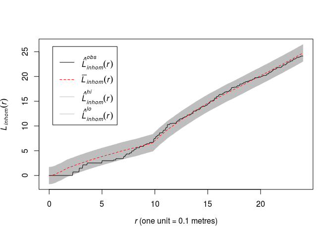
Repeat Question 3 for the inhomogeneous Strauss process with log-quadratic trend, using the inhomogeneous L-function Linhom in place of the usual L-function.
fit2 <- as.ppm(fitp2)
plot(envelope(fit2, Linhom, global = TRUE, nsim = 19, nsim2 = 100), main = "")
## Generating 119 simulated realisations of fitted Gibbs model (100 to
## estimate the mean and 19 to calculate envelopes) ...
## 1, 2, 3, 4.6.8.10.12.14.16.18.20.22.24.26.28.30.32.34.36.38.
## 40.42.44.46.48.50.52.54.56.58.60.62.64.66.68.70.72.74.76.78
## .80.82.84.86.88.90.92.94.96.98.100.102.104.106.108.110.112.114.116.
## 118 119.
##
## Done.