Lab 8: Spacing and distances

This session is concerned with summary statistics for spacings and interpoint distances. The lecturer’s R script is available here (right click and save).

library(spatstat)

Exercise 1

For the swedishpines data:

1. Calculate the estimate of the nearest neighbour distance distribution function G using Gest.

   G <- Gest(swedishpines)
   

2. Plot the estimate of G(r) against r

   plot(G, cbind(km, rs, han) ~ r, main = "Nearest neighbor distance distribution")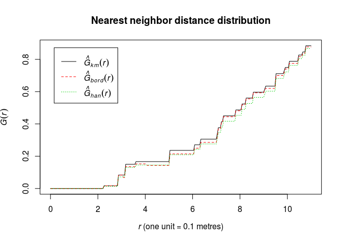
   

   

3. Plot the estimate of G(r) against the theoretical (Poisson) value G_pois(r)=1 − exp(−λπr²).

   E.g.

   plot(G, . ~ theo, main = "Nearest neighbor distribution")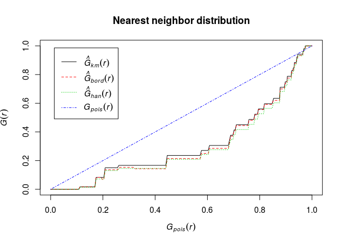
   

   

4. Define Fisher’s variance-stabilising transformation for c.d.f.’s by

   Phi <- function(x) asin(sqrt(x))
   

   Plot the G function using the formula Phi(.) ~ Phi(theo) and interpret it.

   Phi <- function(x) asin(sqrt(x))
   plot(G, Phi(.) ~ Phi(theo), main = "Nearest neighbor distribution")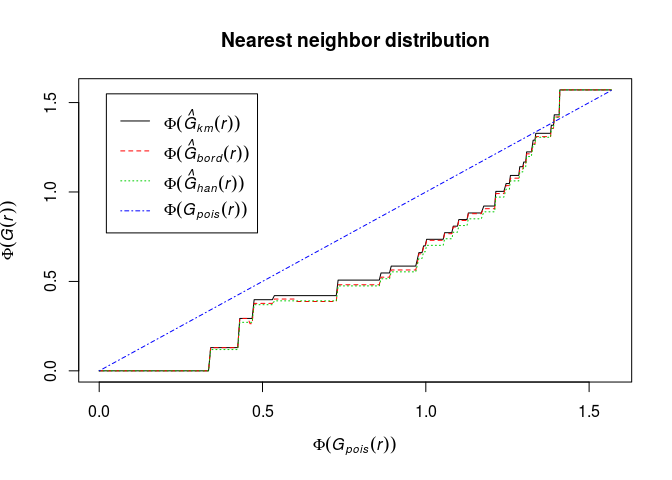
   

   

   The transformation has made the deviations from CSR in the central part of the curve smaller. We need envelopes to say anything about significance.

Exercise 2

For the swedishpines data:

1. Calculate the estimate of the nearest neighbour distance distribution function F using Fest.

   Fhat <- Fest(swedishpines)
   

2. Plot the estimate of F(r) against r

   plot(Fhat, main = "Empty Space function")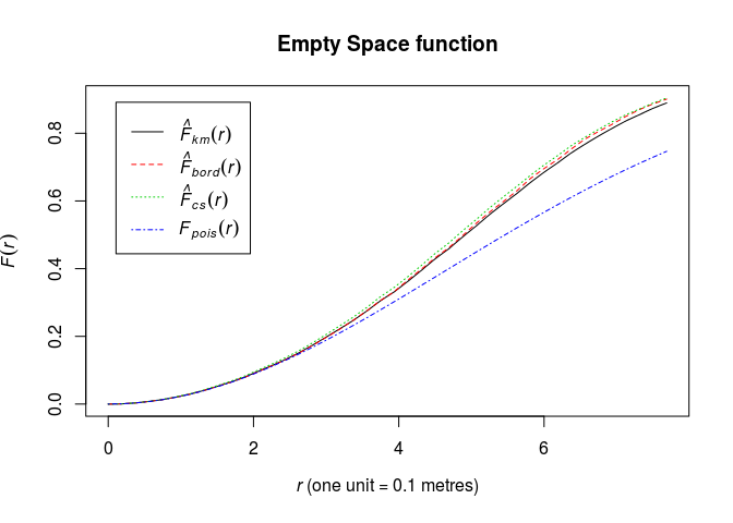
   

   

3. Plot the estimate of F(r) against the theoretical (Poisson) value F_pois(r)=1 − exp(−λπr²).

   plot(Fhat, . ~ theo, main = "")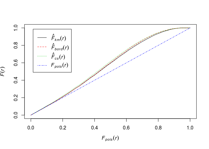
   

   

4. Define Fisher’s variance-stabilising transformation for c.d.f.’s by

   Phi <- function(x) asin(sqrt(x))
   

   Plot the F function using the formula Phi(.) ~ Phi(theo) and interpret it.

   Phi <- function(x) asin(sqrt(x))
   plot(Fhat, Phi(.) ~ Phi(theo), main = "")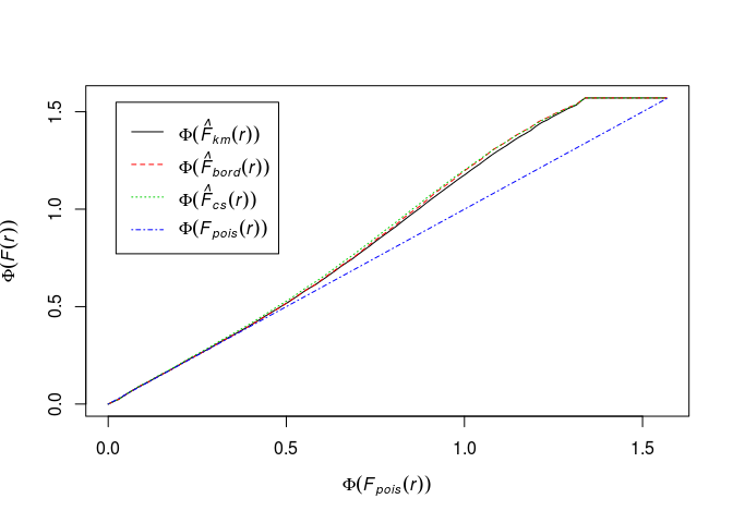
   

   

   The transformation has changed the picture much. It looks like deviation from CSR, but again, without envelopes it’s hard to draw conclusions.