Lab 4: Fitting Poisson models
This session is concerned with Poisson point process models. The lecturer’s R script is available here (right click and save).
library(spatstat)
Exercise 1
The command rpoispp(100) generates realisations of the Poisson process with intensity λ = 100 in the unit square.
-
Repeat the command
plot(rpoispp(100))several times to build your intuition about the appearance of a completely random pattern of points.Let’s plot it three times:
replicate(3, plot(rpoispp(lambda = 100), main = ""))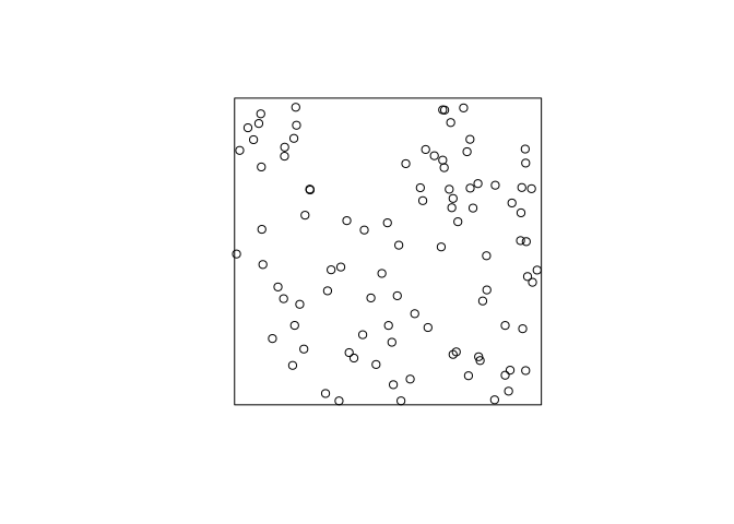
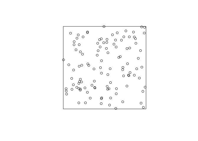
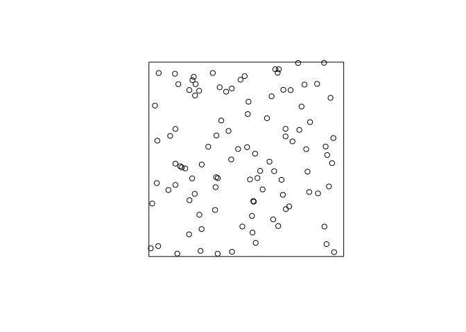
As can be seen, the points (unsurprisingly) are much more random that want one might think. “Randomly” drawing points on a piece of paper one would usually draw a point pattern that is more regular (i.e. the points are repulsive).
-
Try the same thing with intensity λ = 1.5.
For brevity we only do it once here:
plot(rpoispp(lambda = 1.5), main = "")
Here we expect 1.5 points in the plot each time.
Exercise 2
Returning to the Japanese Pines data,
-
Fit the uniform Poisson point process model to the Japanese Pines data
ppm(japanesepines~1)We fit the Poisson process model with the given command and print the output:
m.jp <- ppm(japanesepines ~ 1)
print(m.jp)
## Stationary Poisson process ## Intensity: 65 ## Estimate S.E. CI95.lo CI95.hi Ztest Zval ## log(lambda) 4.174387 0.1240347 3.931284 4.417491 *** 33.65499 -
Read off the fitted intensity. Check that this is the correct value of the maximum likelihood estimate of the intensity.
We extract the coeficient with the
coeffunction, and compare to the straightforward estimate obtained by `intensity``:unname(exp(coef(m.jp)))## [1] 65intensity(japanesepines)## [1] 65As seen, they agree exactly.
Exercise 3
The japanesepines dataset is believed to exhibit spatial inhomogeneity.
-
Plot a kernel smoothed intensity estimate.
Plot the kernel smoothed intensity estimate selecting the bandwidth with
bw.scott:jp.dens <- density(japanesepines, sigma = bw.scott) plot(jp.dens) plot(japanesepines, col = "white", cex = .4, pch = 16, add = TRUE)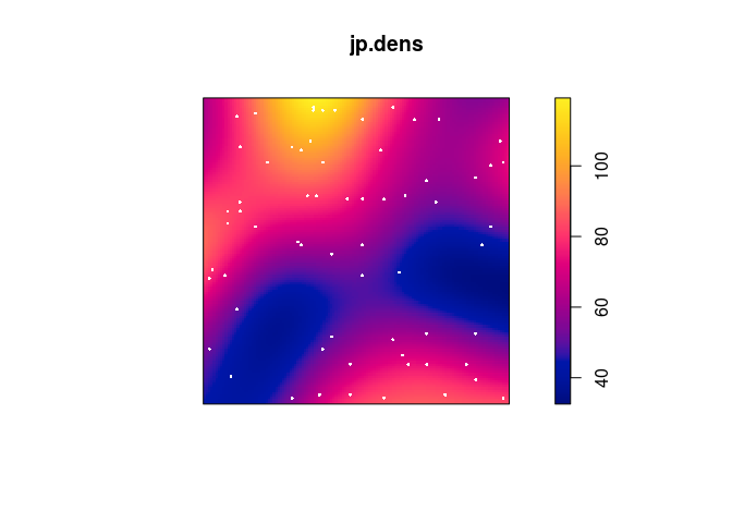
-
Fit the Poisson point process models with loglinear intensity (trend formula
~x+y) and log-quadratic intensity (trend formula~polynom(x,y,2)) to the Japanese Pines data.We fit the two models with
ppm:jp.m <- ppm(japanesepines ~ x + y) jp.m2 <- ppm(japanesepines ~ polynom(x, y, 2) ) -
extract the fitted coefficients for these models using
coef.coef(jp.m)## (Intercept) x y ## 4.0670790 -0.2349641 0.4296171coef(jp.m2)## (Intercept) x y I(x^2) I(x * y) I(y^2) ## 4.0645501 1.1436854 -1.5613621 -0.7490094 -1.2009245 2.5061569 -
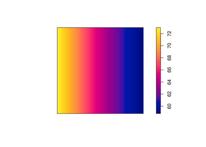
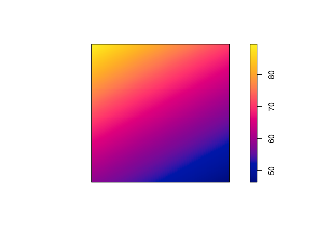
Plot the fitted model intensity (using
plot(predict(fit)))par(mar=rep(0,4)) plot(predict(jp.m), main = "")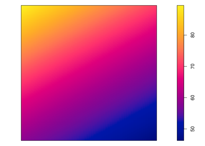
plot(predict(jp.m, se=TRUE)$se, main = "")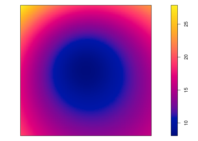
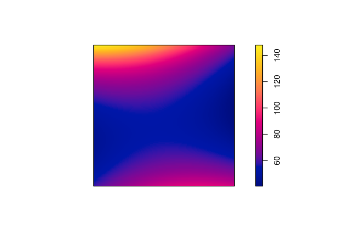
plot(predict(jp.m2), main = "")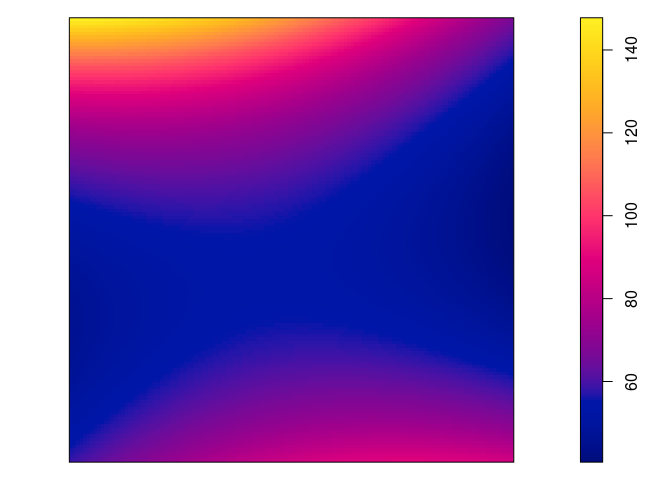
plot(predict(jp.m2, se=TRUE)$se, main = "")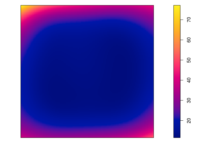
-
perform the Likelihood Ratio Test for the null hypothesis of a loglinear intensity against the alternative of a log-quadratic intensity, using
anova.anova(jp.m, jp.m2)## Analysis of Deviance Table ## ## Model 1: ~x + y Poisson ## Model 2: ~x + y + I(x^2) + I(x * y) + I(y^2) Poisson ## Npar Df Deviance ## 1 3 ## 2 6 3 3.3851 -
Generate 10 simulated realisations of the fitted log-quadratic model, and plot them, using
plot(simulate(fit, nsim=10))wherefitis the fitted model.par(mar=rep(0.5,4)) plot(simulate(jp.m2, nsim=10), main = "")## Generating 10 simulated patterns ...1, 2, 3, 4, 5, 6, 7, 8, 9, 10.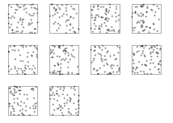
Exercise 4
The update command can be used to re-fit a point process model using a different model formula.
-
Type the following commands and interpret the results:
fit0 <- ppm(japanesepines ~ 1) fit1 <- update(fit0, . ~ x) fit1## Nonstationary Poisson process ## ## Log intensity: ~x ## ## Fitted trend coefficients: ## (Intercept) x ## 4.2895587 -0.2349362 ## ## Estimate S.E. CI95.lo CI95.hi Ztest Zval ## (Intercept) 4.2895587 0.2411952 3.816825 4.7622926 *** 17.7845936 ## x -0.2349362 0.4305416 -1.078782 0.6089098 -0.5456759fit2 <- update(fit1, . ~ . + y) fit2## Nonstationary Poisson process ## ## Log intensity: ~x + y ## ## Fitted trend coefficients: ## (Intercept) x y ## 4.0670790 -0.2349641 0.4296171 ## ## Estimate S.E. CI95.lo CI95.hi Ztest Zval ## (Intercept) 4.0670790 0.3341802 3.4120978 4.7220602 *** 12.1703167 ## x -0.2349641 0.4305456 -1.0788181 0.6088898 -0.5457357 ## y 0.4296171 0.4318102 -0.4167154 1.2759495 0.9949211OK, let’s do that:
fit0 <- ppm(japanesepines ~ 1) fit1 <- update(fit0, . ~ x) fit1## Nonstationary Poisson process ## ## Log intensity: ~x ## ## Fitted trend coefficients: ## (Intercept) x ## 4.2895587 -0.2349362 ## ## Estimate S.E. CI95.lo CI95.hi Ztest Zval ## (Intercept) 4.2895587 0.2411952 3.816825 4.7622926 *** 17.7845936 ## x -0.2349362 0.4305416 -1.078782 0.6089098 -0.5456759fit2 <- update(fit1, . ~ . + y) fit2## Nonstationary Poisson process ## ## Log intensity: ~x + y ## ## Fitted trend coefficients: ## (Intercept) x y ## 4.0670790 -0.2349641 0.4296171 ## ## Estimate S.E. CI95.lo CI95.hi Ztest Zval ## (Intercept) 4.0670790 0.3341802 3.4120978 4.7220602 *** 12.1703167 ## x -0.2349641 0.4305456 -1.0788181 0.6088898 -0.5457357 ## y 0.4296171 0.4318102 -0.4167154 1.2759495 0.9949211 -
Now type
step(fit2)and interpret the results.The backwards selection is done with the code:
step(fit2)## Start: AIC=-407.96 ## ~x + y ## ## Df AIC ## - x 1 -409.66 ## - y 1 -408.97 ## <none> -407.96 ## ## Step: AIC=-409.66 ## ~y ## ## Df AIC ## - y 1 -410.67 ## <none> -409.66 ## ## Step: AIC=-410.67 ## ~1 ## Stationary Poisson process ## Intensity: 65 ## Estimate S.E. CI95.lo CI95.hi Ztest Zval ## log(lambda) 4.174387 0.1240347 3.931284 4.417491 *** 33.65499First, given two models the preferred model is the one with the minimum AIC value. In step 1, the removal of x results in the least AIC and is hence deleted. In step 2, removing y results in a lower AIC than not deleing anything and is thus deleted. This results in the constant model.
Exercise 5
The bei dataset gives the locations of trees in a survey area with additional covariate information in a list bei.extra.
-
Fit a Poisson point process model to the data which assumes that the intensity is a loglinear function of terrain slope and elevation (hint: use
data = bei.extrainppm).We fit the log-linear intensity model with the following:
bei.m <- ppm(bei ~ elev + grad, data = bei.extra) -
Read off the fitted coefficients and write down the fitted intensity function.
The coefficents are extraced with
coef:coef(bei.m)## (Intercept) elev grad ## -8.55862210 0.02140987 5.84104065Hence the model is log**λ(u)= − 8.55 + 0.02 ⋅ E(u)+5.84G(u) where E(u) and G(u) is the elevation and gradient, respectively, at u.
-
Plot the fitted intensity as a colour image.
plot(predict(bei.m), main = "") plot(bei, cex = 0.3, pch = 16, cols = "white", add = TRUE)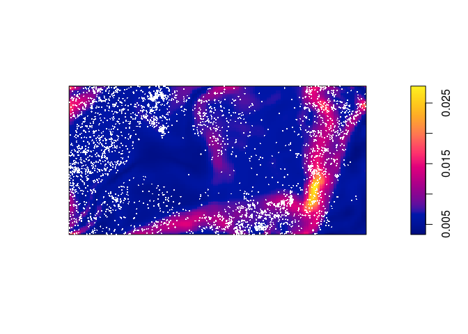
-
extract the estimated variance-covariance matrix of the coefficient estimates, using
vcov.We call
vcovon the fitted model object:vcov(bei.m)## (Intercept) elev grad ## (Intercept) 0.1163496911 -7.774152e-04 -0.0354946468 ## elev -0.0007774152 5.233903e-06 0.0001993179 ## grad -0.0354946468 1.993179e-04 0.0654647795 -
Compute and plot the standard error of the intensity estimate (see
help(predict.ppm)).From the documentation the argument
sewill trigger the computation of the standard errors. These are then plotted in the standard manner.std.err <- predict(bei.m, se = TRUE)$se plot(std.err, main = "")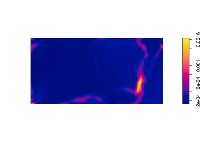
Exercise 6
Fit Poisson point process models to the Japanese Pines data, with the following trend formulas. Read off an expression for the fitted intensity function in each case.
| Trend formula | Fitted intensity function |
|---|---|
~1 |
logλ(u)=4.17 |
~x |
logλ(u)=4.28 − 0.23x |
~sin(x) |
logλ(u)=4.29 − 0.26sin(x) |
~x+y |
logλ(u)=4.07 − 0.23x + 0.42y |
~polynom(x,y,2) |
logλ(u)=4.06 + 1.14x − 1.56y − 0.75x2 − 1.20xy + 2.51y2 |
~factor(x < 0.4) |
logλ(u)=4.10 + 0.16 ⋅ I(x < 0.4) |
(Here, I(⋅) denote the indicator function.)
The fitted intensity functions have been written into the table based on the follwing model fits:
coef(ppm1 <- ppm(japanesepines ~ 1))
## log(lambda)
## 4.174387
coef(ppm2 <- ppm(japanesepines ~ x))
## (Intercept) x
## 4.2895587 -0.2349362
coef(ppm3 <- ppm(japanesepines ~ sin(x)))
## (Intercept) sin(x)
## 4.2915935 -0.2594537
coef(ppm4 <- ppm(japanesepines ~ x + y))
## (Intercept)           x           y
##   4.0670790  -0.2349641   0.4296171
coef(ppm5 <- ppm(japanesepines ~ polynom(x, y, 2)))
## (Intercept)           x           y      I(x^2)    I(x * y)      I(y^2)
##   4.0645501   1.1436854  -1.5613621  -0.7490094  -1.2009245   2.5061569
coef(ppm6 <- ppm(japanesepines ~ factor(x < 0.4)))
##         (Intercept) factor(x < 0.4)TRUE
##           4.1048159           0.1632665
Exercise 7
Make image plots of the fitted intensities for the inhomogeneous models above.
Again, we use plot(predict()):
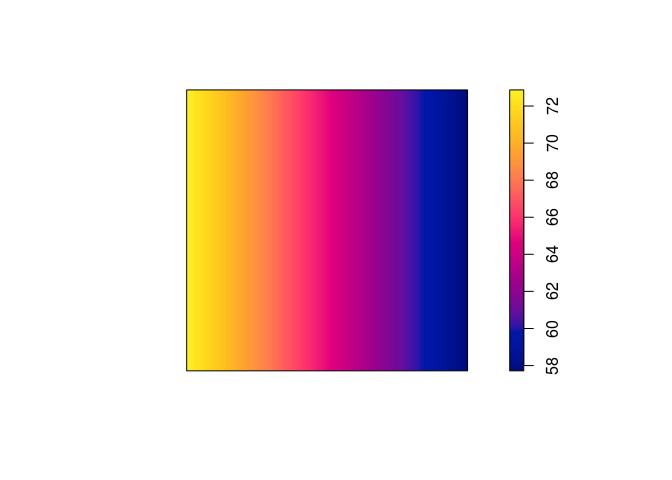
plot(predict(ppm1), main = "")

plot(predict(ppm2), main = "")
plot(predict(ppm3), main = "")
plot(predict(ppm4), main = "")
plot(predict(ppm5), main = "")
plot(predict(ppm6), main = "")