Lab 3: Intensity dependent on covariate

This session covers tools for investigating intensity depending on a covariate. The lecturer’s R script is available here (right click and save).

library(spatstat)

Exercise 1

The bei dataset gives the locations of trees in a survey area with additional covariate information in a list bei.extra.

Assign the elevation covariate to a variable elev by typing
```
elev <- bei.extra$elev
```
OK, lets do that:
```
elev <- bei.extra$elev
```

Plot the trees on top of an image of the elevation covariate.

plot(elev, main = "")
plot(bei, add = TRUE, cex = 0.3, pch = 16, cols = "white")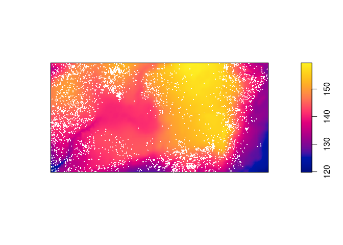

Cut the study region into 4 areas according to the value of the terrain elevation, and make a texture plot of the result.
```
Z <- cut(elev, 4, labels=c("Low", "Med-Low", "Med-High", "High"))
textureplot(Z, main = "")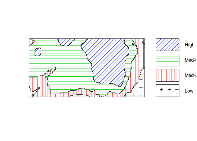
```
Convert the image from above to a tesselation, count the number of points in each region using quadratcount, and plot the quadrat counts.
```
Y <- tess(image = Z)
qc <- quadratcount(bei, tess = Y)
```

Estimate the intensity in each of the four regions.

intensity(qc)

## tile
##         Low     Med-Low    Med-High        High 
## 0.002259007 0.006372523 0.008562862 0.005843516

Exercise 2

Assume that the intensity of trees is a function λ(u)=ρ(e(u)) where e(u) is the terrain elevation at location u.

Compute a nonparametric estimate of the function ρ and plot it by
```
rh <- rhohat(bei, elev)
plot(rh)
```
Repeating the R code:
```
rh <- rhohat(bei, elev)
plot(rh)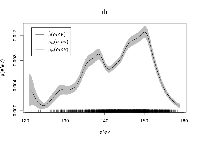
```

Compute the predicted intensity based on this estimate of ρ.

prh <- predict(rh)
plot(prh, main = "")
plot(bei, add = TRUE, cols = "white", cex = .2, pch = 16)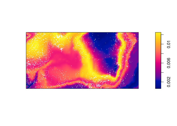

Compute a non-parametric estimate by kernel smoothing and compare with the predicted intensity above.

The kernel density estimate of the points is computed and plotted with the following code:
```
dbei <- density(bei, sigma = bw.scott)
plot(dbei, main = "")
plot(bei, add = TRUE, cols = "white", cex = .2, pch = 16)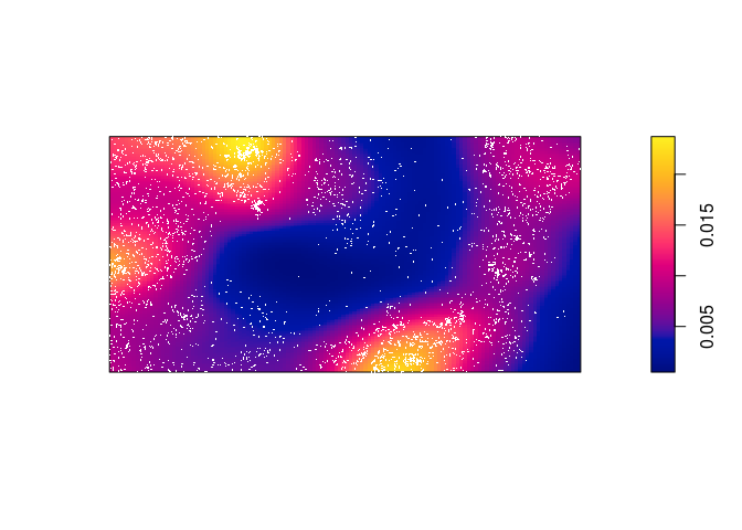
```
Which seems to be quite different form the predicted intentisty.

Bonus info: To plot the two intensity estimates next to each other you collect the estimates as a spatial object list (solist) and plot the result (the estimates are called pred and ker below):

l <- solist(pred, ker)
plot(l, equal.ribbon = TRUE, main = "", 
     main.panel = c("rhohat prediction", "kernel smoothing"))

l <- solist(prh, dbei)
plot(l, equal.ribbon = TRUE, main = "",
     main.panel = c("rhohat prediction", "kernel smoothing"))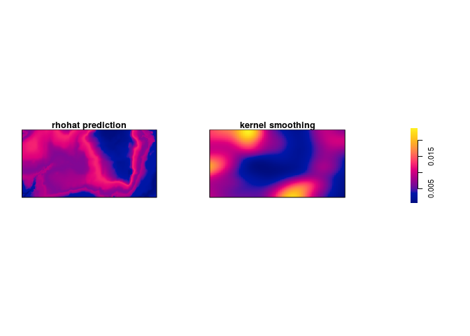

Exercise 3

Continuing with the dataset bei conduct both Berman’s Z1 and Z2 tests for dependence on elev, and plot the results.

The tests are done straightforwardly with berman.test:

Z1 <- berman.test(bei, elev)
print(Z1)

## 
##  Berman Z1 test of CSR in two dimensions
## 
## data:  covariate 'elev' evaluated at points of 'bei'
## Z1 = -0.72924, p-value = 0.4659
## alternative hypothesis: two-sided

plot(Z1)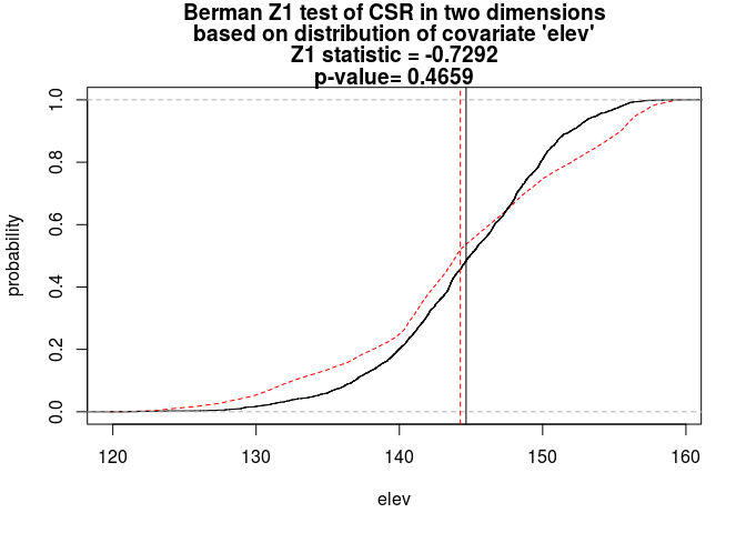

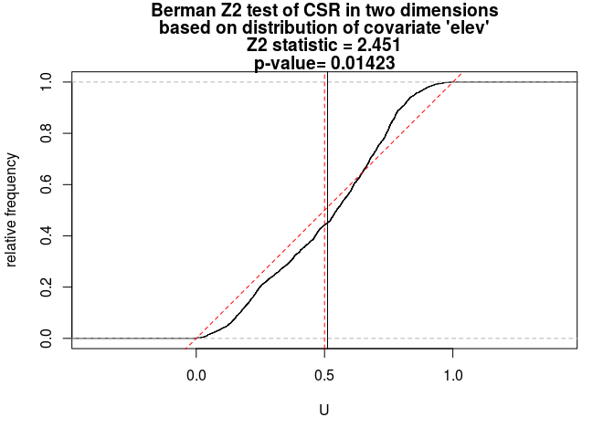
Z2 <- berman.test(bei, elev, which = "Z2")
print(Z2)

## 
##  Berman Z2 test of CSR in two dimensions
## 
## data:  covariate 'elev' evaluated at points of 'bei' 
##   and transformed to uniform distribution under CSR
## Z2 = 2.4515, p-value = 0.01423
## alternative hypothesis: two-sided

plot(Z2)