Lab 1: Introduction

This session is about reading in, displaying and summarising point patterns. The lecturer’s R script is available here (right click and save).

If you have not already done so, you’ll need to start R and load the spatstat package by typing

library(spatstat)

Exercise 1

We will study a dataset that records the locations of Ponderosa Pine trees (Pinus ponderosa) in a study region in the Klamath National Forest in northern California. The data are included with spatstat as the dataset ponderosa.

assign the data to a shorter name, like X or P;

To assign the data to X we simply write:
```
X <- ponderosa
```
plot the data;

To plot the data we do the following:
```
plot(X)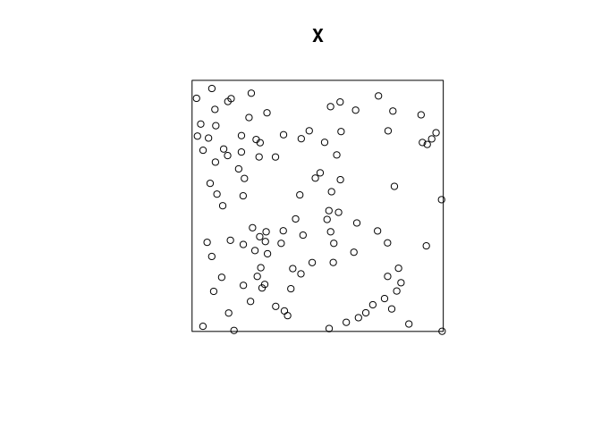
```
By the S3 method dispatch, this calls the plot.ppp function. The chars argument indicate that the point type should be be periods (“.”).
find out how many trees are recorded;

Both npoints and print.ppp displays the number of recorded trees:
```
npoints(X)
```
```
## [1] 108
```
```
print(X)
```
```
## Planar point pattern: 108 points
## window: rectangle = [0, 120] x [0, 120] metres
```
I.e. there are 108 trees in the dataset.
find the dimensions of the study region;

The dimensions of the observation window can be seen above. Alternatively, it can be directly assesed via
```
window(X)
```
```
## Planar point pattern: 5 points
## window: rectangle = [0, 120] x [0, 120] metres
```

obtain an estimate of the average intensity of trees (number of trees per unit area).

The average intensity can be computed via intensity.ppp

intensity(X)

## [1] 0.0075

or the more expansive summary.ppp:

summary(X)

## Planar point pattern:  108 points
## Average intensity 0.0075 points per square metre
## 
## Coordinates are given to 3 decimal places
## i.e. rounded to the nearest multiple of 0.001 metres
## 
## Window: rectangle = [0, 120] x [0, 120] metres
## Window area = 14400 square metres
## Unit of length: 1 metre

Exercise 2

The Ponderosa data, continued:

When you type plot(ponderosa), the command that is actually executed is plot.ppp, the plot method for point patterns. Read the help file for the function plot.ppp, and find out which argument to the function can be used to control the main title for the plot;

From the documentation, the argument that controls the title is main as is also the case in the regular generic plot.
plot the Ponderosa data with the title Ponderosa Pine Trees above it;
```
plot(ponderosa, main = "Ponderosa Pine Trees")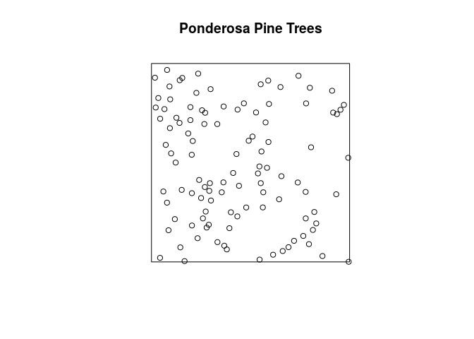
```
from your reading of the help file, predict what will happen if we type
```
plot(ponderosa, chars="X", cols="green")
```
then check that your guess was correct;

Each point will be plotted as an green “X” and indeed:
```
plot(ponderosa, chars="X", cols="green")
```
try different values of the argument chars, for example, one of the integers 0 to 25, or a letter of the alphabet. (Note the difference between chars=3 and chars="+", and the difference between chars=4 and chars="X").

There are subtle differences in the actual character/point types plotted. When given a string literal, the actual character is plotted as the point type.
```
plot(ponderosa, chars=3, cols="green")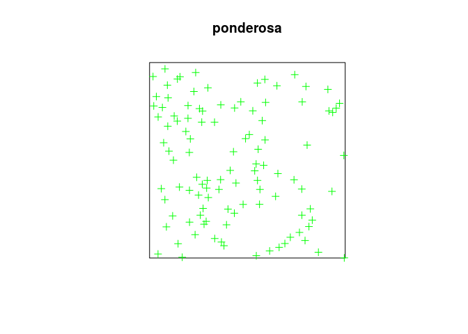
```
```
plot(ponderosa, chars="+", cols="green")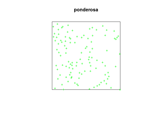
```
```
plot(ponderosa, chars=4, cols="green")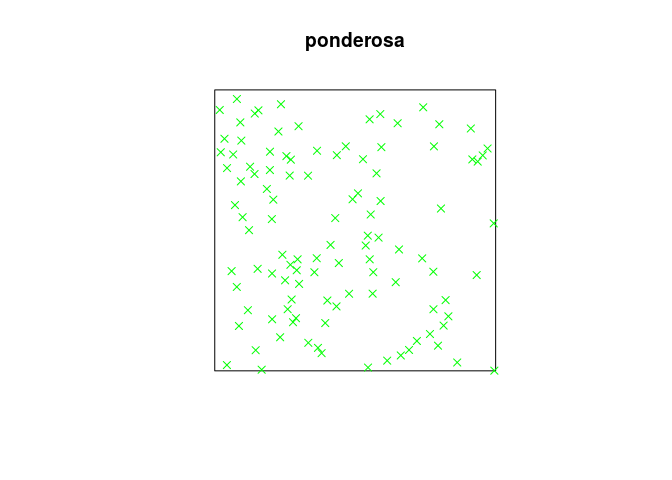
```
```
plot(ponderosa, chars="X", cols="green")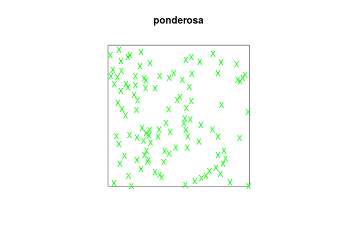
```

Exercise 3

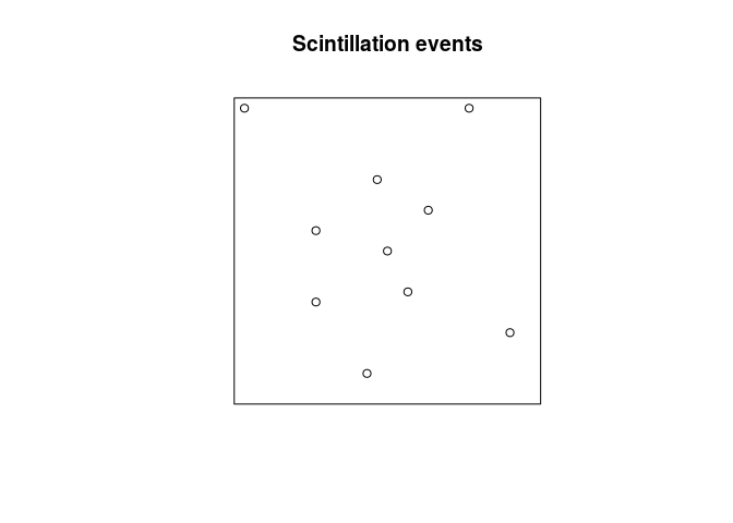
The following vectors record the locations of 10 scintillation events observed under a microscope. Coordinates are given in microns, and the study region was 30 × 30 microns, with the origin at the bottom left corner.

x <- c(13, 15, 27, 17, 8, 8, 1, 14, 19, 23)
y <- c(3, 15, 7, 11, 10, 17, 29, 22, 19, 29)

Create a point pattern X from the data, and plot the point pattern (use owin or square to define the study region).

To define the observation window we do:

w <- owin(c(0, 30), c(0, 30), unitname = c("micron", "microns"))

With this window, we create the ppp object with the funciton of the same name and plot it:

P <- ppp(x = x, y = y, window = w)
plot(P, main = "Scintillation events")

Exercise 4

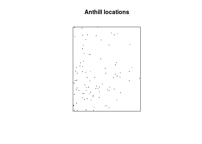
The file anthills.txt is available in the Data directory on GitHub and downloadable by this direct link (right click and save).

It records the locations of anthills recorded in a 1200x1500 metre study region in northern Australia. Coordinates are given in metres, along with a letter code recording the ecological ‘status’ of each anthill (in this exercise we will ignore this letter code).

read the data into R as a data frame, using the R function read.table. (Since the input file has a header line, you will need to use the argument header=TRUE when you call read.table.)

We read the data into R with the line:
```
dat <- read.table(file = "../Data/anthills.txt", header = TRUE)
```
check the data for any peculiarities.

Looking at the first entries of the dataset with
```
head(dat)
```
```
##     x    y status
## 1 105  372      j
## 2  65  142      g
## 3 132  862      f
## 4  22   19      g
## 5 185 1173      e
## 6  69  557      f
```
We see that there is a status variable indicating that this is a marked point process.
create a point pattern hills containing these data. Ensure that the unit of length is given its correct name.

As before
```
hills <- with(dat, ppp(x, y, xrange = c(0, 1200), yrange = c(0, 1500), 
                       units=c("metre", "metres")))
```
The ppp function passes the appropriate arguments to owin which we therefore do not need to call explicitly.

plot the data.

As before, we can now plot the data:

plot(hills, pch = 16, cex = 0.3, main = "Anthill locations")