Melb2018

Lab 5: Marked point patterns

This session covers modelling of marked point patterns using marked point processes. The lecturer’s R script is available here (right click and save).

library(spatstat)

Exercise 1

The dataset spruces contains the Norwegian Spruces dataset giving the locations of trees and their diameters at breast height.

Read the help file for the data;
access the dataset and plot it;
```
plot(spruces)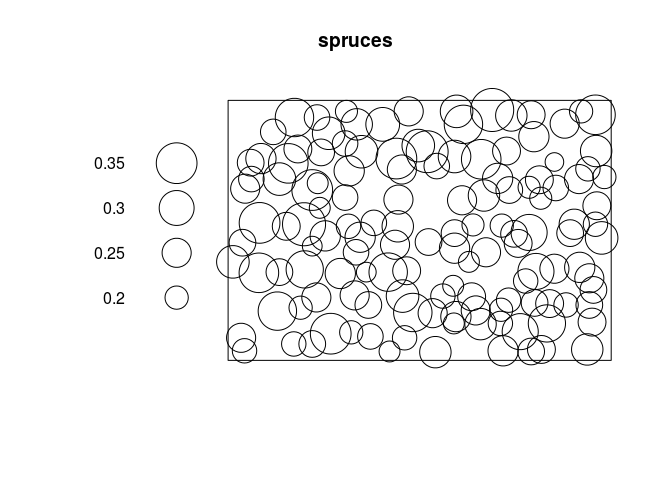
```
re-plot the data so that the tree diameters are displayed at a physical scale that is 10 times the physical scale of the location coordinates.
```
plot(spruces, markscale = 10)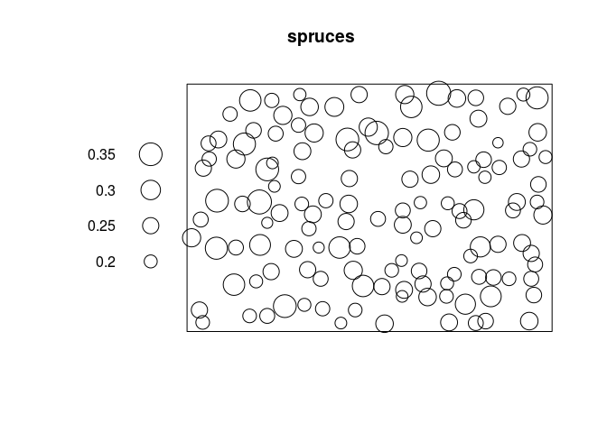
```
use Smooth (notice the upper case S) to compute and plot a pixel image of the local average tree diameter;
```
plot(Smooth(spruces, sigma = 8))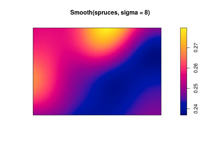
```
trees are normally classified as ‘adult’ when their diameter exceeds 30 centimetres. Use the cut command to classify each tree as adult or juvenile, and produce a multitype point pattern in which the trees are marked as adult or juvenile. Plot this pattern, and plot the adults and juveniles separately.
```
cutspruces <- cut(spruces, breaks = c(0,0.3,0.4), labels = c("juvenile", "adult"))
plot(cutspruces, main = "")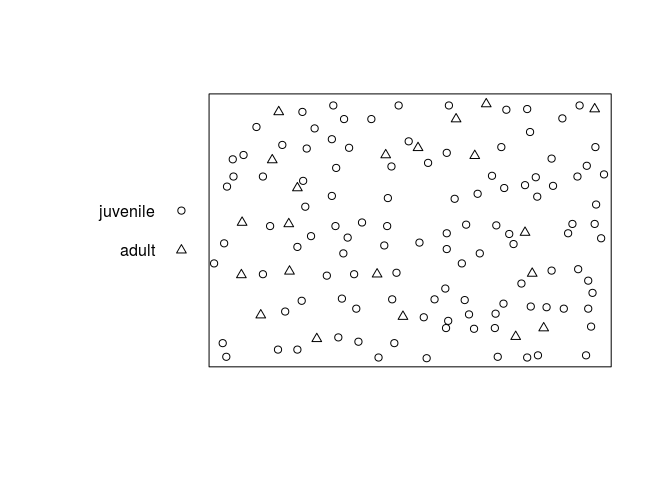
```
```
plot(split(cutspruces), main = "")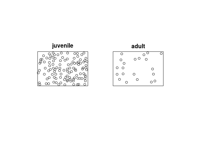
```

Exercise 2

The file anthills.txt is available in the Data directory on github and downloadable by this direct link (right click and save).

It records the locations of anthills recorded in a 1200x1500 metre study region in northern Australia. Coordinates are given in metres, along with a letter code recording the ecological ‘status’ of each anthill.

read the data into R as a data frame, using the R function read.table. (Since the input file has a header line, you will need to use the argument header=TRUE when you call read.table.)
```
dat <- read.table(file = "../Data/anthills.txt", header = TRUE)
```
check the data for any peculiarities.

create a point pattern hills containing these data. Ensure that the marks are a factor, and that the unit of length is given its correct name.

hills <- with(dat, ppp(x, y, xrange = c(0, 1200), yrange = c(0, 1500),
                       marks = status, units=c("metre", "metres")))

plot the data.
```
plot(hills, main = "")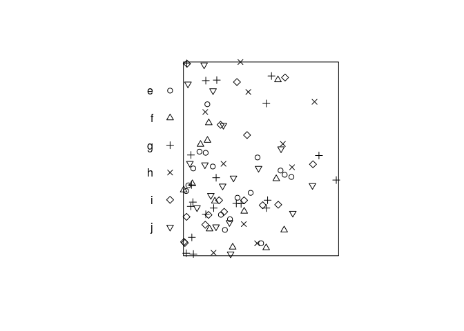
```

Exercise 3

The dataset hamster is a multitype pattern representing the locations of cells of two types, dividing and pyknotic.

plot the data;
```
plot(hamster)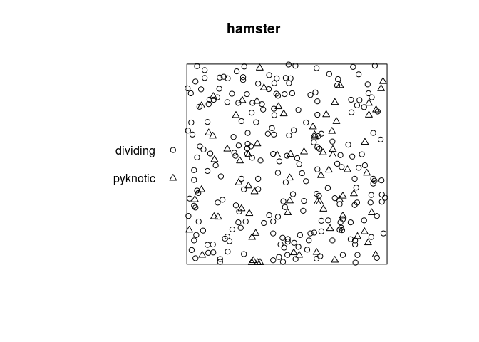
```
plot the patterns of pyknotic and dividing cells separately;
```
plot(split(hamster), main = "")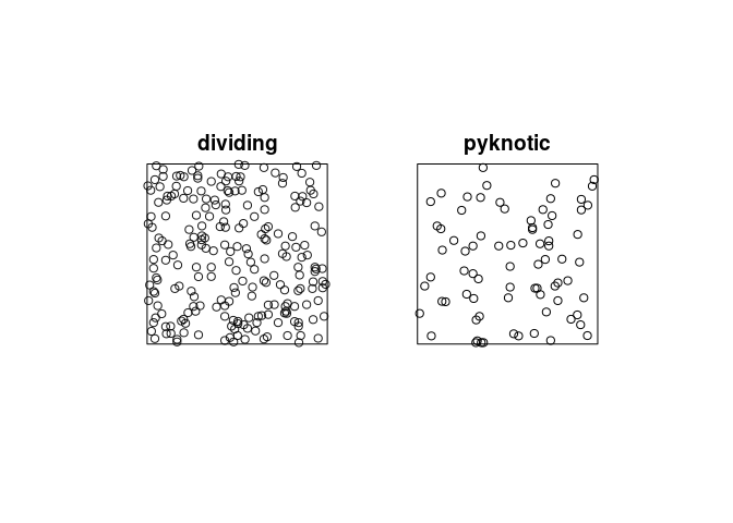
```
plot kernel estimates of the intensity functions of pyknotic and dividing cells separately;
```
plot(density(split(hamster)), main = "")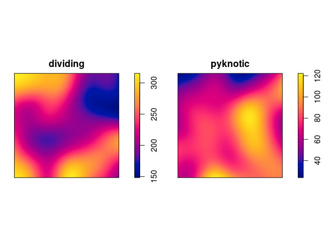
```
use relrisk to perform cross-validated bandwidth selection and computation of the relative intensity of pyknotic cells.
```
plot(relrisk(hamster, hmax = 1, relative = TRUE, control = "dividing"))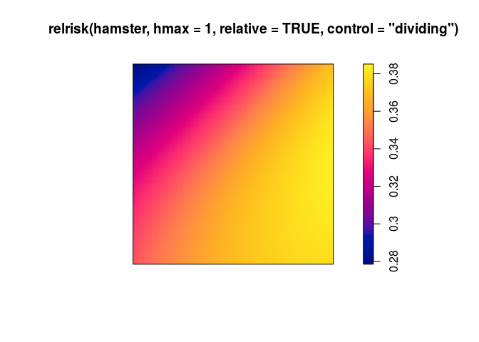
```

Exercise 4

The command rmpoispp generates simulated realisations of a multitype Poisson process. The first argument lambda specifies the intensity function (\lambda(x,y,m)) which gives the intensity of points at location (x,y). It may be given in several forms.

If lambda is a single number, it specifies the intensity of points of each type. Try computing, inspecting and plotting the result of

rmpoispp(21, win=square(1), types=c("yes", "no"))

What is the expected total number of points generated by this command?

X <- rmpoispp(21, win=square(1), types=c("yes", "no"))
summary(X)

## Marked planar point pattern:  32 points
## Average intensity 32 points per square unit
## 
## Coordinates are given to 8 decimal places
## 
## Multitype:
##     frequency proportion intensity
## yes        20      0.625        20
## no         12      0.375        12
## 
## Window: rectangle = [0, 1] x [0, 1] units
## Window area = 1 square unit

plot(X, main = "")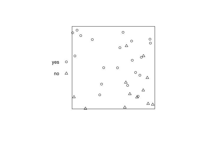

We expect (2\times21=42) points on average.

If lambda is a vector of numbers, the vector entries specify the intensities for each type of point. Try
```
rmpoispp(c(20,40,20), types=letters[1:3])
```
What is the expected total number of points generated by this command?
```
rmpoispp(c(20,40,20), types=letters[1:3])
```
We expect (20+40+20=80) points on average in this case.
If lambda is a function with arguments x,y,m then this is interpreted as the intensity function (\lambda(x,y,m)). Try
```
fun <- function(x,y,m) { 40 * (x+y) }
X <- rmpoispp(fun, types=letters[24:26])
fun2 <- function(x,y,m) { ifelse(m == "yes", 100 * x, 50 * (1-x)) }
X2 <- rmpoispp(fun2, types=c("yes", "no"))
```
What is the expected total number of points in X?

We expect (3\cdot\int_{[0,1]}\int_{[0,1]} 40 (x+y) d!x!d!y = 120) points on average in this case.

Exercise 5

Take the Harkness-Isham ants’ nests data ants

use summary to estimate the average intensities of the points of each type.

summary(ants)

## Marked planar point pattern:  97 points
## Average intensity 0.0002261486 points per square unit (one unit = 0.5 
## feet)
## 
## Coordinates are integers
## i.e. rounded to the nearest unit (one unit = 0.5 feet)
## 
## Multitype:
##             frequency proportion    intensity
## Cataglyphis        29  0.2989691 6.761144e-05
## Messor             68  0.7010309 1.585372e-04
## 
## Window: polygonal boundary
## single connected closed polygon with 11 vertices
## enclosing rectangle: [-25, 803] x [-49, 717] units
## Window area = 428922 square units
## Unit of length: 0.5 feet
## Fraction of frame area: 0.676

lam <- intensity(ants)

Generate and plot a realisation of a marked Poisson process in the same window as the data, with the same possible types of points, with uniform intensities for each type, given by the intensities estimated from the data.

rmpoispp(lam, win = Window(ants), types = names(lam))

## Marked planar point pattern: 92 points
## Multitype, with levels = Cataglyphis, Messor 
## window: polygonal boundary
## enclosing rectangle: [-25, 803] x [-49, 717] units (one unit = 0.5 feet)

Or the even shorter

rmpoispp(lam, win = Window(ants))

## Marked planar point pattern: 110 points
## Multitype, with levels = Cataglyphis, Messor 
## window: polygonal boundary
## enclosing rectangle: [-25, 803] x [-49, 717] units (one unit = 0.5 feet)

Repeat the simulation several times. Do the simulations look like the data?

Make 11 simulations:
```
simants <- rmpoispp(lam, win = Window(ants), types = names(lam), nsim = 11)
```
Add original data as list item number 12:
```
simants[[12]] <- ants
```
Plot them all:
```
plot(simants, legend = FALSE, main = "")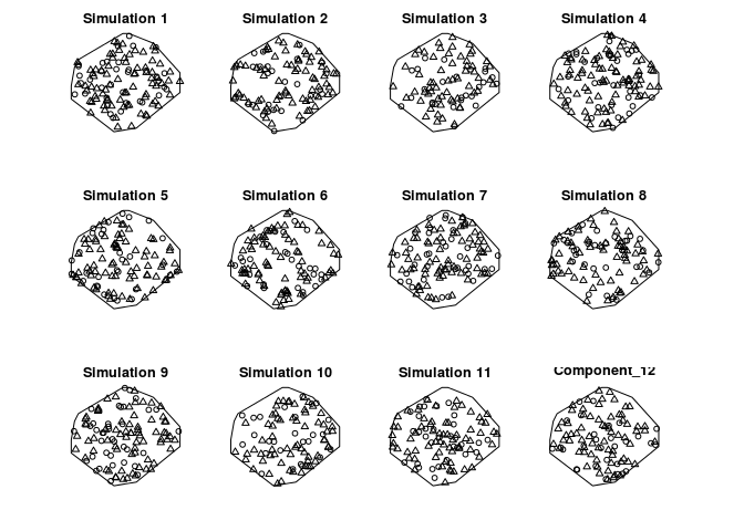
```

Exercise 6

Here we will fit multitype Poisson point process models to the Harkness-Isham ants’ nests data ants.

Fit the model ppm(ants ~ marks) and interpret the result. Compare the result with summary(ants) and explain the similarities.

fit1 <- ppm(ants ~ marks)

This is a Poisson model with a separate constant intensity for each mark. The fitted intensities are:

exp(coef(fit1)[1])

##  (Intercept) 
## 6.762949e-05

exp(coef(fit1)[1] + coef(fit1)[2])

##  (Intercept) 
## 0.0001585795

This agrees perfectly with the output of summary(ants):

summary(ants)

## Marked planar point pattern:  97 points
## Average intensity 0.0002261486 points per square unit (one unit = 0.5 
## feet)
## 
## Coordinates are integers
## i.e. rounded to the nearest unit (one unit = 0.5 feet)
## 
## Multitype:
##             frequency proportion    intensity
## Cataglyphis        29  0.2989691 6.761144e-05
## Messor             68  0.7010309 1.585372e-04
## 
## Window: polygonal boundary
## single connected closed polygon with 11 vertices
## enclosing rectangle: [-25, 803] x [-49, 717] units
## Window area = 428922 square units
## Unit of length: 0.5 feet
## Fraction of frame area: 0.676

Fit the model ppm(ants ~ marks + x) and write down an expression for the fitted intensity function.
```
fit2 <- ppm(ants ~ marks + x)
(co <- coef(fit2))
```
```
##   (Intercept)   marksMessor             x 
## -9.5243832518  0.8522118655 -0.0002041438
```
Intensity for the reference type (Cataglyphis):

[\lambda( (x,y) ) = \exp(-9.5243833 + -2.0414381\times 10^{-4} \cdot x)]

Intensity for the other type (Messor):

[\lambda( (x,y) ) = \exp(-9.5243833 + 0.8522119 + -2.0414381\times 10^{-4} \cdot x)]
Fit the model ppm(ants ~ marks * x) and write down an expression for the fitted intensity function.
```
fit3 <- ppm(ants ~ marks * x)
(co <- coef(fit3))
```
```
##   (Intercept)   marksMessor             x marksMessor:x 
## -9.605698e+00  9.676854e-01  1.107981e-05 -3.071343e-04
```
Intensity for the reference type (Cataglyphis):

[\lambda( (x,y) ) = \exp(-9.605698 + 1.1079805\times 10^{-5} \cdot x)]

Intensity for the other type (Messor):

[\lambda( (x,y) ) = \exp(-9.605698 + 0.9676854 + (1.1079805\times 10^{-5} + 0.9676854) \cdot x)]

Compute the fitted intensities of the three models fitted above using predict and plot the results.

pred <- c(predict(fit1), predict(fit2), predict(fit3))
plot(as.solist(pred), ncols = 2, main = "")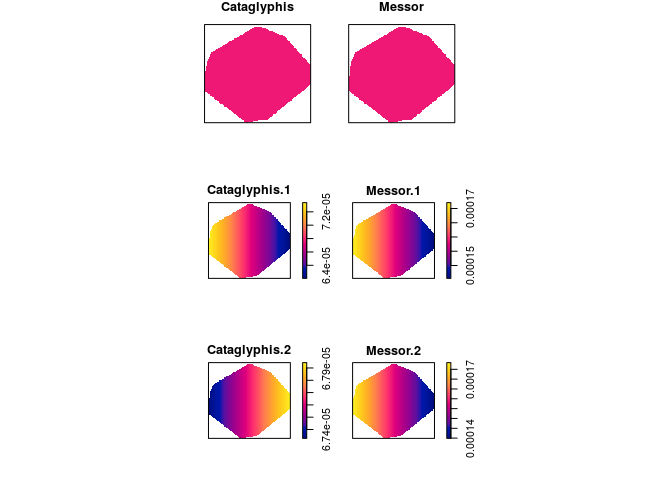

Explain the difference between the models fitted by ppm(ants ~ marks + x) and ppm(ants ~ marks * x) .

For the additive model the effect of the x coordinate is the same for both types of ants, while the effect of x differs in the multiplicative model.

Exercise 7

The study region for the ants’ nests data ants is divided into areas of ‘scrub’ and ‘field’. We want to fit a Poisson model with different intensities in the field and scrub areas.

The coordinates of two points on the boundary line between field and scrub are given in ants.extra$fieldscrub. First construct a function that determines which side of the line we are on:

fs <- function(x,y) {
  ends <- ants.extra$fieldscrub
  angle <- atan(diff(ends$y)/diff(ends$x))
  normal <- angle + pi/2
  project <- (x - ends$x[1]) * cos(normal) + (y - ends$y[1]) * sin(normal)
  factor(ifelse(project > 0, "scrub", "field"))
}

Now fit the models:

ppm(ants ~ marks + side, data = list(side=fs))
ppm(ants ~ marks * side, data = list(side=fs))

and interpret the results.

fit1 <- ppm(ants ~ marks + side, data = list(side=fs))
fit2 <- ppm(ants ~ marks * side, data = list(side=fs))

In the first model the fitted intensity is lower in the scrub than in the field (but this effect is not significant).

In the second model the fitted intensity of Cataglyphis is lower in the scrub than the intensity of Cataglyphis in the field, where as it is the other way around for Messor. When we allow for the different effect between ant types the scrub/field covariate is significant.

This site is open source. Improve this page.