ECAS2019

Lab 3: Dependence – solution

This session covers tools for investigating dependence between points.

library(spatstat)

Exercise 1

The swedishpines dataset was recorded in a study plot in a large forest. We shall assume the pattern is stationary.

Calculate the estimate of the $K$ -function using Kest.

The estimation is done with:
```
K <- Kest(swedishpines)
```
Plot the estimate of $K(r)$ against $r$

To plot the K-function, we do:
```
plot(K, main = "K-function")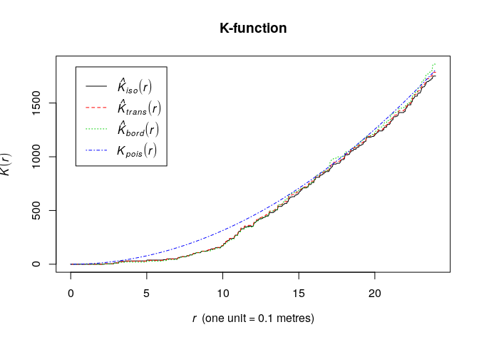
```
Plot the estimate of $K(r) - \pi\!r^2$ against $r$ (Hint: look at the fmla argument in plot.fv).

The estimated K-function subtracted $\pi\!r^2$ can be done via the fmla (formula) interface:
```
plot(K, . - pi*r^2 ~ r, main = "Normalized K-function",
     legendpos = "bottomright")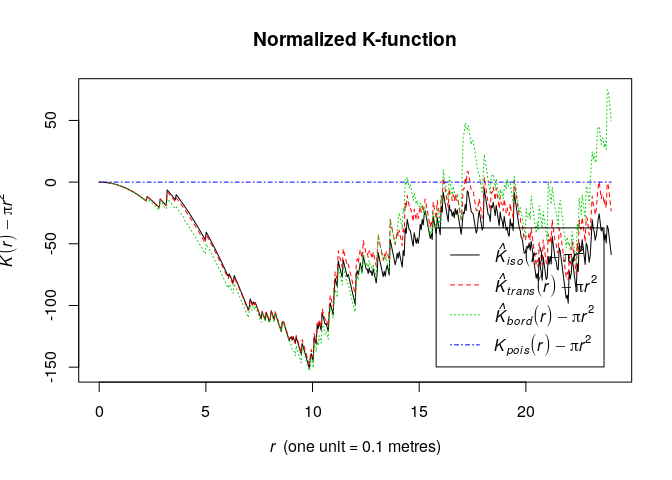
```
Calculate and plot an estimate of the pair correlation function using pcf.

The pair-correlation is also compute straight-forwardly:
```
pcorf <- pcf(swedishpines)
plot(pcorf)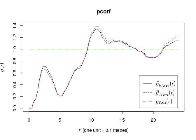
```
Draw tentative conclusions from these plots about interpoint interaction in the data.

Assuming a homogeneous point pattern, both the L- and K-function are less what is expected under the Poisson process the data. Thus they indicate a comparatively regular point pattern. Similarly, the pair-correlation function also suggests this.

Exercise 2

The command rThomas generates simulated realisations of the Thomas model (‘modified Thomas cluster process’).

Read the help file.

See help("rThomas").
Type plot(rThomas(10, 0.05, 8)) a few times, and interpret the results.
```
replicate(3, plot(rThomas(10, 0.05, 8), main = ""))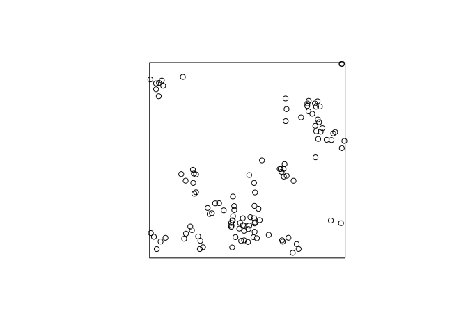
```
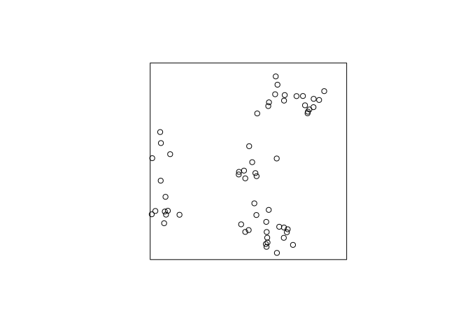
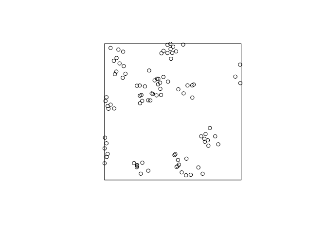
A clustered process – on average 10 clusters with 8 points. The standard deviation of the cluster distribution is 0.05, so most points will be within distance 0.10 from their parent.
Experiment with the arguments of rThomas to obtain point patterns that
1. consist of a few, well-separated, very tight clusters of points;
2. look similar to realisations of a uniform Poisson process.
We get few clusters by reducing the intensity of the parent process (first argument). Tightly and separated clusters are obtained by reducing the standard deviation (second argument).
```
plot(rThomas(5, scale = 0.01, mu = 8), main = "")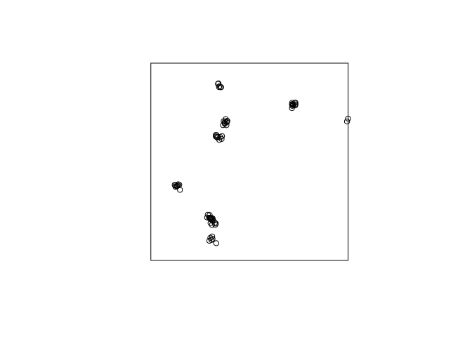
```
If the are many clusters with a large standard deviation it looks like Poisson.
```
plot(rThomas(100, scale = 1, mu = 1), main = "")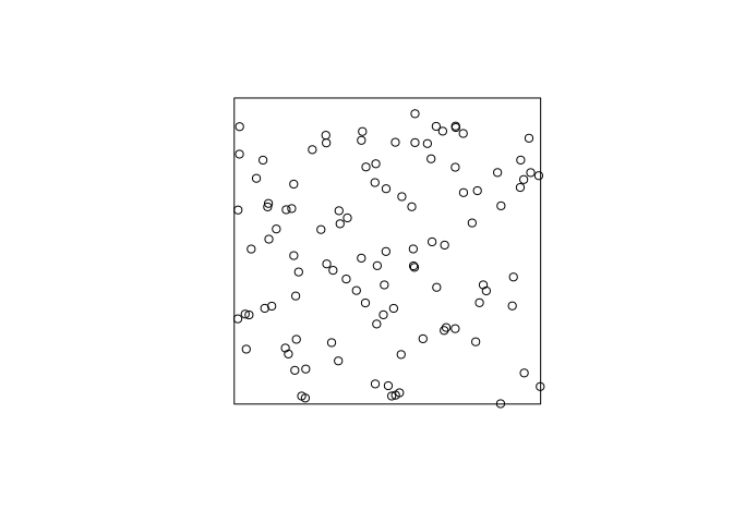
```

Exercise 3

Read the help file for kppm.

See help("kppm").

Fit the Thomas model to the redwood data by the method of minimum contrast:

fit <- kppm(redwood ~ 1, clusters="Thomas")
fit
plot(fit)

From the documentation, the minmum contrast fitting procedure is default. Hence, we need not specify it.

fit <- kppm(redwood ~ 1, clusters = "Thomas")
fit

## Stationary cluster point process model
## Fitted to point pattern dataset 'redwood'
## Fitted by minimum contrast
##  Summary statistic: K-function
## 
## Uniform intensity:   62
## 
## Cluster model: Thomas process
## Fitted cluster parameters:
##      kappa      scale 
## 23.5511449  0.0470461 
## Mean cluster size:  2.632568 points

plot(fit, main = "", pause = FALSE)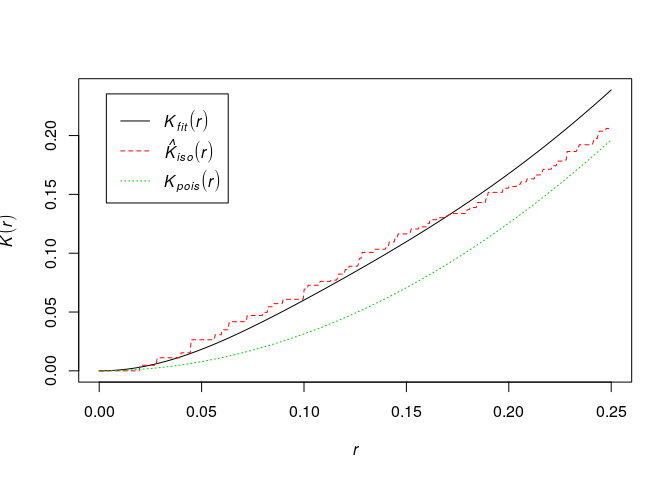 

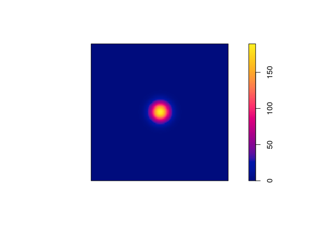
Read off the parameters of the fitted model, and generate a simulated realisation of the fitted model using rThomas.

From the previous output, we can read off the parameters to do the simulation (or we can use parameters to extract them):
```
(p <- parameters(fit))
```
```
## $trend
## [1] 62
## 
## $kappa
## [1] 23.55114
## 
## $scale
## [1] 0.0470461
## 
## $mu
## [1] 2.632568
```
```
rt2 <- rThomas(kappa = p$kappa, scale = p$scale, mu = p$mu)
plot(rt2, main = "")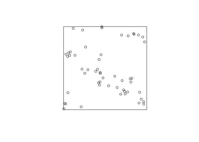
```
Type plot(simulate(fit)) to generate a simulated realisation of the fitted model automatically.

OK, let try that alternative:
```
plot(simulate(fit, drop = TRUE), main = "")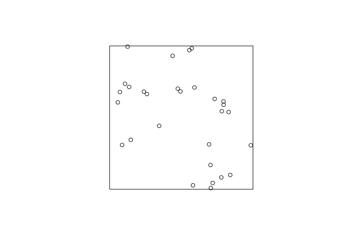
```

Try the command

fit2 <- kppm(redwood ~ 1, clusters="Thomas", startpar=c(kappa=10, scale=0.1))

and briefly explore the fitting algorithm’s sensitivity to the initial guesses at the parameter values kappa and scale.

For “large” kappa (parent intensity) and “small” scale (standard deviation), the algorithm seems quite robust:

kppm(redwood ~ 1, clusters="Thomas", startpar=c(kappa=10, scale=0.1))

## Stationary cluster point process model
## Fitted to point pattern dataset 'redwood'
## Fitted by minimum contrast
##  Summary statistic: K-function
## 
## Uniform intensity:   62
## 
## Cluster model: Thomas process
## Fitted cluster parameters:
##       kappa       scale 
## 23.54757642  0.04704921 
## Mean cluster size:  2.632967 points

kppm(redwood ~ 1, clusters="Thomas", startpar=c(kappa=100, scale=0.01))

## Stationary cluster point process model
## Fitted to point pattern dataset 'redwood'
## Fitted by minimum contrast
##  Summary statistic: K-function
## 
## Uniform intensity:   62
## 
## Cluster model: Thomas process
## Fitted cluster parameters:
##       kappa       scale 
## 23.54962713  0.04705395 
## Mean cluster size:  2.632738 points

However, for a very small parent intensity (kappa) and large offspring scale the fit changes considerably.

kppm(redwood ~ 1, clusters="Thomas", startpar=c(kappa=0.1, scale=10))

## Stationary cluster point process model
## Fitted to point pattern dataset 'redwood'
## Fitted by minimum contrast
##  Summary statistic: K-function
## 
## Uniform intensity:   62
## 
## Cluster model: Thomas process
## Fitted cluster parameters:
##       kappa       scale 
## 0.001824317 9.427722055 
## Mean cluster size:  33985.33 points

Generate and plot several simulated realisations of the fitted model, to assess whether it is plausible.
```
XX <- simulate(fit, nsim = 11)
```
```
## Generating 11 simulations... 1, 2, 3, 4, 5, 6, 7, 8, 9, 10,  11.
## Done.
```
```
XX[[12]] <- redwood
plot(XX, main = "", main.panel = "")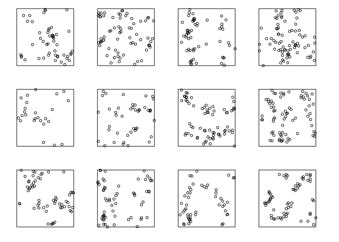
```
The actual data do not look too different from the simulated (apart from the artificial discretisation in the real data which can be seen on larger plots).

Extract and plot the fitted pair correlation function by

pcffit <- pcfmodel(fit)
plot(pcffit, xlim = c(0, 0.3))

OK, let’s try that:

pcffit <- pcfmodel(fit)
plot(pcffit, xlim = c(0, 0.3), main = "pair correlation")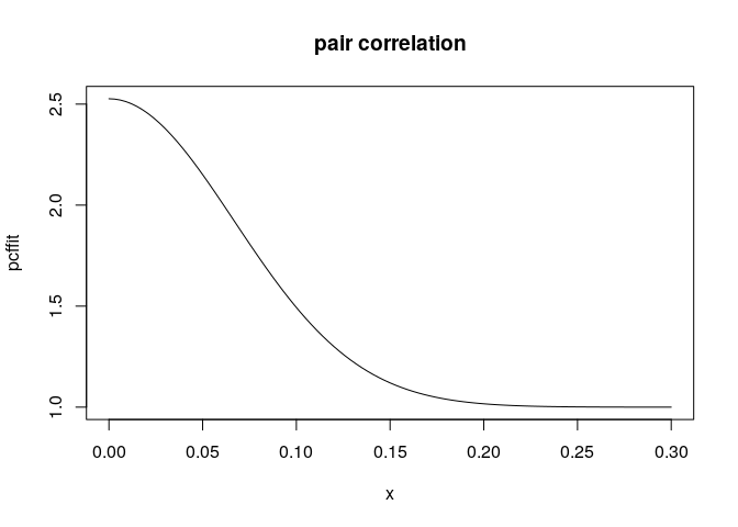

Type plot(envelope(fit, Lest, nsim=39)) to generate simulation envelopes of the $L$ function from this fitted model. Do they suggest the model is plausible?

plot(envelope(fit, Lest, nsim = 39, global = TRUE))

## Generating 78 simulated realisations of fitted cluster model (39 to 
## estimate the mean and 39 to calculate envelopes) ...
## 1, 2, 3, 4, 5, 6, 7, 8, 9, 10, 11, 12, 13, 14, 15, 16, 17, 18, 19, 20, 21, 22, 23, 24, 25, 26, 27, 28, 29, 30, 31, 32, 33, 34, 35, 36, 37, 38,
## 39, 40, 41, 42, 43, 44, 45, 46, 47, 48, 49, 50, 51, 52, 53, 54, 55, 56, 57, 58, 59, 60, 61, 62, 63, 64, 65, 66, 67, 68, 69, 70, 71, 72, 73, 74, 75, 76,
## 77,  78.
## 
## Done.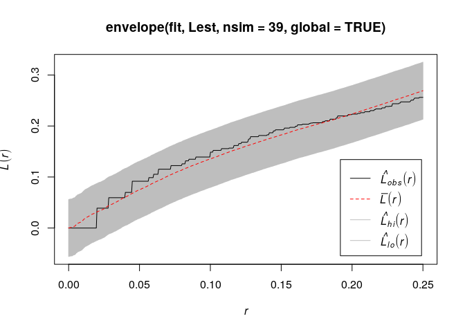

Yes, the model seems plausible and it does not devivate from the envelope.

Exercise 4

Fit a Matern cluster process to the redwood data.

We fit the Matern cluster process by specifying the clusters argument to be MatClust.
```
mfit <- kppm(redwood ~ 1, clusters = "MatClust")
```
Use vcov to estimate the covariance matrix of the parameter estimates.

The variance (covariance matrix) is computed straightforwardly:
```
vcov(mfit)
```
```
##             (Intercept)
## (Intercept)  0.05304008
```
Compare with the covariance matrix obtained when fitting a homogeneous Poisson model.
```
vcov(ppm(redwood ~ 1))
```
```
##             log(lambda)
## log(lambda)  0.01612903
```
As can be seen, the variance of the intensity estimate is quite a bit larger in the Matern model. This comes naturally by the doubly stochastic construction of the Matern model.

Exercise 5

In this question we fit a Strauss point process model to the swedishpines data.

We need a guess at the interaction distance $R$ . Compute and plot the $K$ -function of the dataset and choose the value $r$ which maximises the discrepancy $|K(r)-\pi r^2|$ .

We plot the above function which we want to maximize.
```
plot(Kest(swedishpines), abs(iso - theo) ~ r, main = "")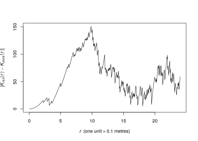
```
As seen from the plot, the maximum lies around $r = 9$ by eye. We find the optimum explicitly like follows:
```
discrep <- function(r) {
  return(abs(as.function(Kest(swedishpines))(r) - pi*r^2))
}
res <- optimise(discrep, interval = c(0.1, 20), maximum = TRUE)
print(res)
```
```
## $maximum
## [1] 9.84372
## 
## $objective
## [1] 150.6897
```
```
R <- res$maximum
```
This corresponds nicely with the plot.
Fit the stationary Strauss model with the chosen interaction distance using
```
ppm(swedishpines ~ 1, Strauss(R))
```
where R is your chosen value.

As we have assigned R, we simply write:
```
fit <- ppm(swedishpines ~ 1, Strauss(R))
```

Interpret the printout: how strong is the interaction?

print(fit)

## Stationary Strauss process
## 
## First order term:  beta = 0.08310951
## 
## Interaction distance:    9.84372
## Fitted interaction parameter gamma:   0.2407279
## 
## Relevant coefficients:
## Interaction 
##   -1.424088 
## 
## For standard errors, type coef(summary(x))

As seen, the $\gamma = `round(exp(coef(fit)[2]), 2)$ parameter is quite small. Thus there seems to be a strong negative association between points within distance R of each other. A $\gamma$ of $0$ implies the hard core process whereas $\gamma = 1$ implies the Poisson process and thus CSR.

Plot the fitted pairwise interaction function using plot(fitin(fit)).

The pairwise interaction function become:
```
plot(fitin(fit))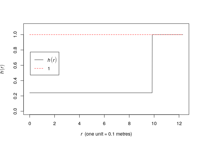
```

Exercise 6

In Question 5 we guesstimated the Strauss interaction distance parameter. Alternatively this parameter could be estimated by profile pseudolikelihood.

Look again at the plot of the $K$ -function of swedishpines and determine a plausible range of possible values for the interaction distance.
```
plot(Kest(swedishpines), main = "")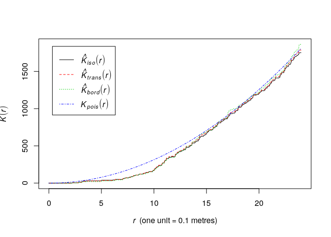
```
A conservative range of plausible interaction distances seems to be 5 to 12 meters.
Generate a sequence of values equally spaced across this range, for example, if your range of plausible values was $[0.05, 0.3]$ , then type
```
rvals <- seq(0.05, 0.3, by=0.01)
```
We generate the numbers between 5 and 12.
```
rvals <- seq(5, 12, by = 0.1)
```
Construct a data frame, with one column named r (matching the argument name of Strauss), containing these values. For example
```
D <- data.frame(r = rvals)
```
OK,
```
D <- data.frame(r = rvals)
```

Execute

fitp <- profilepl(D, Strauss, swedishpines ~ 1)

to find the maximum profile pseudolikelihood fit.

OK, let’s execute it:

fitp <- profilepl(D, Strauss, swedishpines ~ 1)

## (computing rbord)

## comparing 71 models...

## 1, 2, 3, 4, 5, 6, 7, 8, 9, 10, 11, 12, 13, 14, 15, 16, 17, 18, 19, 20, 21, 22, 23, 24, 25, 26, 27, 28, 29, 30, 31, 32, 33, 34, 35, 36, 37, 38,
## 39, 40, 41, 42, 43, 44, 45, 46, 47, 48, 49, 50, 51, 52, 53, 54, 55, 56, 57, 58, 59, 60, 61, 62, 63, 64, 65, 66, 67, 68, 69, 70,  71.

## fitting optimal model...

## done.

Print and plot the object fitp.

print(fitp)

## profile log pseudolikelihood
## for model:  ppm(swedishpines ~ 1,  interaction = Strauss)
## fitted with rbord = 12
## interaction: Strauss process
## irregular parameter: r in [5, 12]
## optimum value of irregular parameter:  r = 9.8

plot(fitp)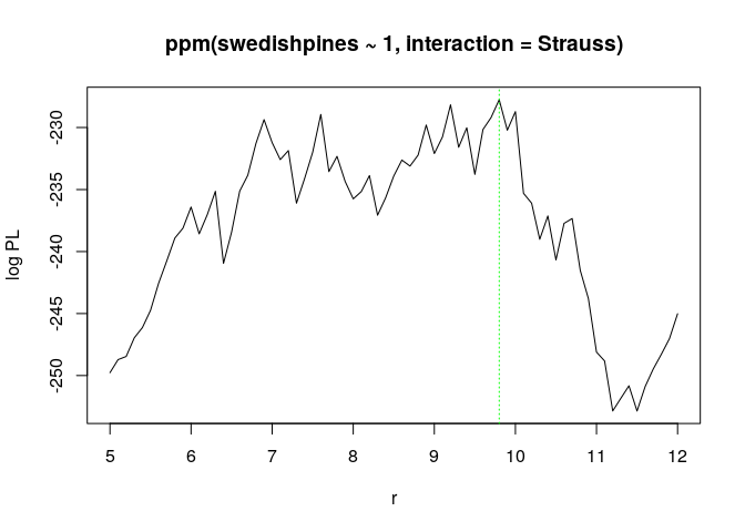

Compare the computed estimate of interaction distance $r$ with your guesstimate. Compare the corresponding estimates of the Strauss interaction parameter $\gamma$ .
```
(Ropt <- reach(as.ppm(fitp)))
```
```
## [1] 9.8
```
The $r = 9.8$ is consistent with the previous guesstimate.
Extract the fitted Gibbs point process model from the object fitp as
```
bestfit <- as.ppm(fitp)
```
OK, let’s do that:
```
bestfit <- as.ppm(fitp)
```

Exercise 7

Modify Question 5 by using the Huang-Ogata approximate maximum likelihood algorithm (method="ho") instead of maximum pseudolikelihood (the default, method="mpl").

fit.mpl <- ppm(swedishpines ~ 1, Strauss(R), method = "mpl")
fit.ho  <- ppm(swedishpines ~ 1, Strauss(R), method = "ho")

## Simulating... 1, 2, 3, 4, 5, 6, 7, 8, 9, 10, 11, 12, 13, 14, 15, 16, 17, 18, 19, 20, 21, 22, 23, 24, 25, 26, 27, 28, 29, 30, 31, 32, 33, 34, 35, 36, 37, 38,
## 39, 40, 41, 42, 43, 44, 45, 46, 47, 48, 49, 50, 51, 52, 53, 54, 55, 56, 57, 58, 59, 60, 61, 62, 63, 64, 65, 66, 67, 68, 69, 70, 71, 72, 73, 74, 75, 76,
## 77, 78, 79, 80, 81, 82, 83, 84, 85, 86, 87, 88, 89, 90, 91, 92, 93, 94, 95, 96, 97, 98, 99,  100.
## Done.

print(fit.ho)

## Stationary Strauss process
## 
## First order term:  beta = 0.1076896
## 
## Interaction distance:    9.84372
## Fitted interaction parameter gamma:   0.2198154
## 
## Relevant coefficients:
## Interaction 
##   -1.514967 
## 
## For standard errors, type coef(summary(x))

print(fit.mpl)

## Stationary Strauss process
## 
## First order term:  beta = 0.08310951
## 
## Interaction distance:    9.84372
## Fitted interaction parameter gamma:   0.2407279
## 
## Relevant coefficients:
## Interaction 
##   -1.424088 
## 
## For standard errors, type coef(summary(x))

The fits are very similar.

Exercise 8

Repeat Question 6 for the inhomogeneous Strauss process with log-quadratic trend. The corresponding call to profilepl is

fitp <- profilepl(D, Strauss, swedishpines ~ polynom(x,y,2))

## (computing rbord)

## comparing 71 models...

## 1, 2, 3, 4, 5, 6, 7, 8, 9, 10, 11, 12, 13, 14, 15, 16, 17, 18, 19, 20, 21, 22, 23, 24, 25, 26, 27, 28, 29, 30, 31, 32, 33, 34, 35, 36, 37, 38,
## 39, 40, 41, 42, 43, 44, 45, 46, 47, 48, 49, 50, 51, 52, 53, 54, 55, 56, 57, 58, 59, 60, 61, 62, 63, 64, 65, 66, 67, 68, 69, 70,  71.

## fitting optimal model...

## done.

fitp2 <- profilepl(D, Strauss, swedishpines ~ polynom(x,y,2))

## (computing rbord)

## comparing 71 models...

## 1, 2, 3, 4, 5, 6, 7, 8, 9, 10, 11, 12, 13, 14, 15, 16, 17, 18, 19, 20, 21, 22, 23, 24, 25, 26, 27, 28, 29, 30, 31, 32, 33, 34, 35, 36, 37, 38,
## 39, 40, 41, 42, 43, 44, 45, 46, 47, 48, 49, 50, 51, 52, 53, 54, 55, 56, 57, 58, 59, 60, 61, 62, 63, 64, 65, 66, 67, 68, 69, 70,  71.

## fitting optimal model...

## done.

print(fitp2)

## profile log pseudolikelihood
## for model:  ppm(swedishpines ~ polynom(x,  y,  2),  interaction = Strauss)
## fitted with rbord = 12
## interaction: Strauss process
## irregular parameter: r in [5, 12]
## optimum value of irregular parameter:  r = 9.8

(bestfit <- as.ppm(fitp2))

## Nonstationary Strauss process
## 
## Log trend:  ~x + y + I(x^2) + I(x * y) + I(y^2)
## 
## Fitted trend coefficients:
##   (Intercept)             x             y        I(x^2)      I(x * y) 
## -5.156605e+00  4.269469e-02  8.582459e-02 -5.324026e-06 -7.955428e-04 
##        I(y^2) 
## -5.506409e-04 
## 
## Interaction distance:    9.8
## Fitted interaction parameter gamma:   0.2390264
## 
## Relevant coefficients:
## Interaction 
##   -1.431181 
## 
## For standard errors, type coef(summary(x))

reach(bestfit)

## [1] 9.8