ECAS2019

Notes for session 2

Adrian Baddeley and Ege Rubak July 15, 2019

Intensity

Often the main objective is to study the “density” of points in the point pattern and to investigate any spatial variation in this density.

Point processes

In a statistical approach to data analysis, we think of the observed data as the outcome of a random process.

To analyse spatial point pattern data, we will regard the observed point pattern $x$ as a realisation of a random point process $X$ .

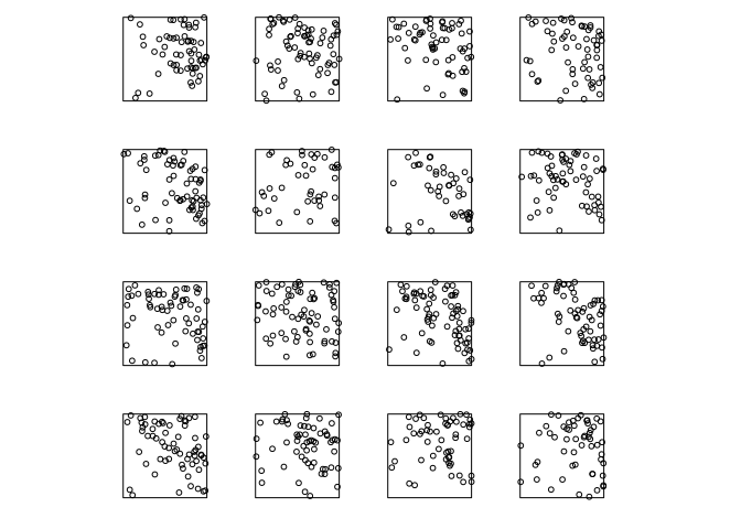
It is helpful to visualise a point process as a collection (“ensemble”) of many different possible outcomes. Here is one example:

Intensity

The intensity of a point process is the expected number of points per unit area. It may be a constant $\lambda \ge 0$ , or it may be spatially varying.

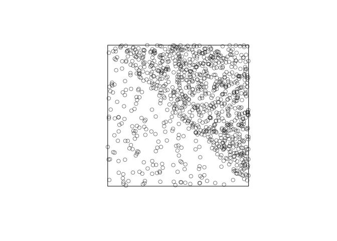
Intensity is an average, over all possible outcomes of the point process. We can visualise it by superimposing the ensemble of outcomes:

We will usually assume that the point process has an intensity function $\lambda(u)$ defined at every spatial location $u$ . Then $\lambda(u)$ is the spatially-varying expected number of points per unit area. It is formally defined to satisfy
$E[ n(B \cap X) ] = \int_B \lambda(u) \, {\rm d}u$
for any region $B \subset R^2$ , where $n(B \cap X)$ denotes the number of points falling in $B$ .

Intensity is closely related to probability density. If $X$ is a point process with intensity function $\lambda(u)$ , then each individual point inside $W$ has probability density $f(u) = \lambda(u)/\Lambda_W$ , where $\Lambda_W = \int_W \lambda(u) \, {\rm d}u$ .

Nonparametric estimation

Because of the close relationship between intensity and probability density, methods for nonparametric estimation of the intensity function are very similar to methods for density estimation.

Nonparametric estimation of spatially-varying intensity

Given a point pattern $x = \{ x_1, \ldots, x_n \}$ in a window $W$ the kernel estimate of intensity is
$\widehat\lambda(u) = \sum_{i=1}^n k(u - x_i) e(u, x_i)$
where $k(x)$ is the smoothing kernel and $e(u, v)$ is a correction for edge effects.

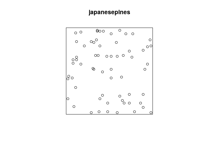
library(spatstat)
plot(japanesepines)

Z <- density(japanesepines, sigma=0.1)
plot(Z)

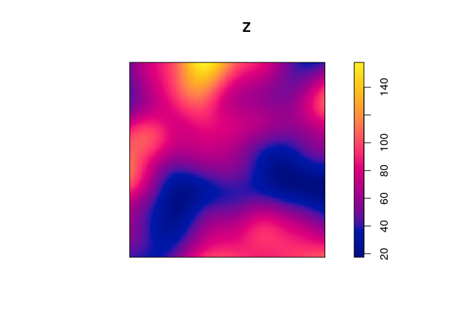
The command in spatstat to compute the kernel estimate of intensity is density.ppp, a method for the generic function density.

The argument sigma is the bandwidth of the smoothing kernel.

Bandwidth can be selected automatically:

bw.ppl(japanesepines)

##     sigma 
## 0.7071068

bw.diggle(japanesepines)

##      sigma 
## 0.05870841

bw.scott(japanesepines)

##   sigma.x   sigma.y 
## 0.1415691 0.1567939

Nonparametric estimation of spatially-varying, mark-dependent intensity

A marked point pattern, with marks which are categorical values, effectively classifies the points into different types.

mucosa

## Marked planar point pattern: 965 points
## Multitype, with levels = ECL, other 
## window: rectangle = [0, 1] x [0, 0.81] units

plot(mucosa, cols=c(2,3))

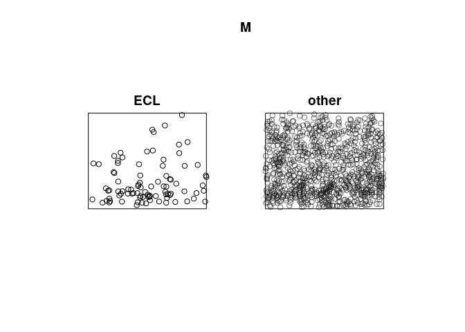
Extract the sub-patterns of points of each type:

M <- split(mucosa)
M

## Point pattern split by factor 
## 
## ECL:
## Planar point pattern: 89 points
## window: rectangle = [0, 1] x [0, 0.81] units
## 
## other:
## Planar point pattern: 876 points
## window: rectangle = [0, 1] x [0, 0.81] units

class(M)

## [1] "splitppp" "ppplist"  "solist"   "list"

plot(M)

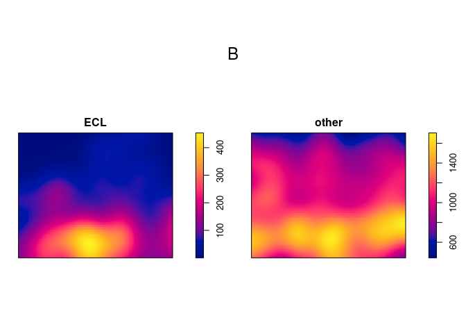
Apply kernel smoothing to each sub-pattern using density.splitppp:

B <- density(M, sigma=bw.ppl)
B

## List of pixel images
## 
## ECL:
## real-valued pixel image
## 128 x 128 pixel array (ny, nx)
## enclosing rectangle: [0, 1] x [0, 0.81] units
## 
## other:
## real-valued pixel image
## 128 x 128 pixel array (ny, nx)
## enclosing rectangle: [0, 1] x [0, 0.81] units

plot(B)

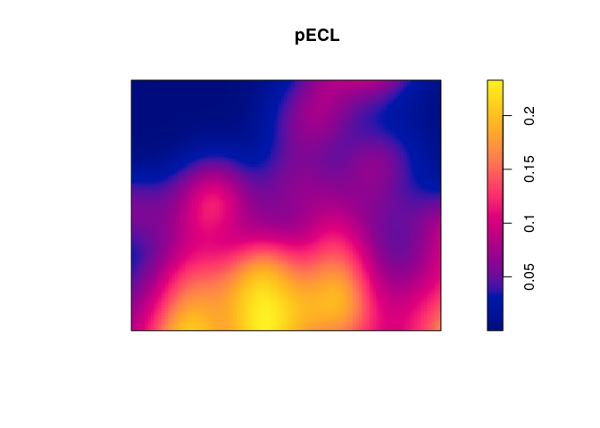
Suppose $\lambda_i(u)$ is the intensity function of the points of type $i$ , for $i=1,2,\ldots,m$ . The intensity function of all points regardless of type is
$\lambda_{\bullet}(u) = \sum_{i=1}^m \lambda_i(u).$
Under reasonable assumptions, the probability that a random point at location $u$ belongs to type $i$ is
$p_i(u) = \frac{\lambda_i(u)}{\lambda_{\bullet}(u)}.$
We could calculate this by hand in spatstat:

lambdaECL <- B[["ECL"]]
lambdaOther <- B[["other"]]
lambdaDot <- lambdaECL + lambdaOther
pECL <- lambdaECL/lambdaDot
pOther <- lambdaOther/lambdaDot
plot(pECL)

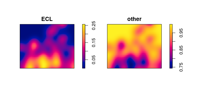
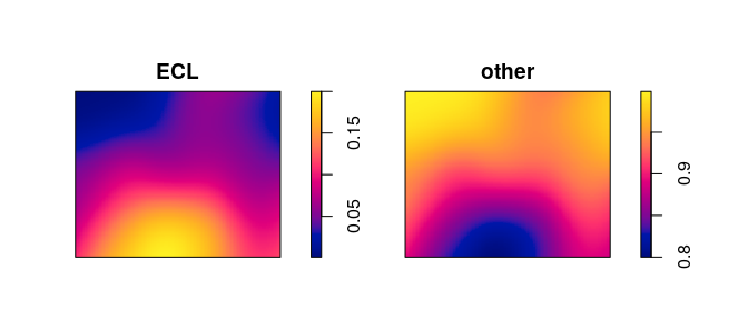
These calculations are automated in the function relrisk (relative risk):

V <- relrisk(mucosa, bw.ppl, casecontrol=FALSE)
plot(V, main="")

Bandwidth selection for the ratio is different from bandwidth selection for the intensity. We recommend using the special algorithm bw.relrisk:

bw.relrisk(mucosa)

##     sigma 
## 0.1282096

Vr <- relrisk(mucosa, bw.relrisk, casecontrol=FALSE)
plot(Vr, main="")

Segregation of types

“Segregation” occurs if the probability distribution of types of points is spatially varying.

A Monte Carlo test of segregation can be performed using the nonparametric estimators described above. The function segregation.test performs it.

segregation.test(mucosa, sigma=0.15, verbose=FALSE)

## 
##  Monte Carlo test of spatial segregation of types
## 
## data:  mucosa
## T = 0.33288, p-value = 0.45

Nonparametric estimation of intensity depending on a covariate

In some applications we believe that the intensity depends on a spatial covariate $Z$ , in the form

$\lambda(u) = \rho(Z(u))$
where $\rho(z)$ is an unknown function which we want to estimate. A nonparametric estimator of $\rho$ is
$\hat\rho(z) = \frac{\sum_{i=1}^n k(Z(x_i) - z)}{\int_W k(Z(u) - z) \, {\rm d} u}$
where $k()$ is a one-dimensional smoothing kernel. This is computed by rhohat.

Example: mucosa data, enterochromaffin-like cells (ECL)

E <- split(mucosa)$ECL
plot(E)

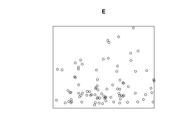
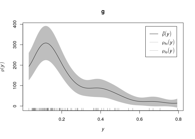
The wall of the gut is at the bottom of the picture. Cell density appears to decline as we go further away from the wall. Use the string "y" to refer to the $y$ coordinate:

g <- rhohat(E, "y")
plot(g)

Example: Murchison gold survey.

X <- murchison$gold
L <- murchison$faults
X <- rescale(X, 1000, "km")
L <- rescale(L, 1000, "km")
D <- distfun(L)
plot(solist(gold=X, faults=L, distance=D), main="", equal.scales=TRUE)

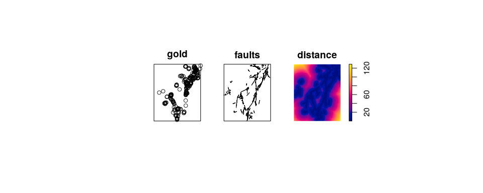
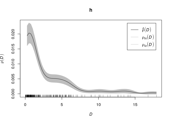
Gold deposits are frequently found near a geological fault line. Here we converted the fault line pattern into a spatial covariate
$D(u) = \mbox{ distance from } u \mbox{ to nearest fault }$

h <- rhohat(X, D)
plot(h)

Parametric modelling

We can formulate a parametric model for the intensity and fit it to the point pattern data, using the spatstat function ppm (point process model).

In its simplest form, ppm fits a Poisson point process model to the point pattern data.

Poisson point process

The homogeneous Poisson process with intensity $\lambda > 0$ in two-dimensional space is characterised by the following properties:

for any region $B$ , the random number $n(X \cap B)$ of points falling in $B$ follows a Poisson distribution;
for any region $B$ , the expected number of points falling in $B$ is $E[n(X \cap B)] = \lambda \, \mbox{area}(B)$ ;
for any region $B$ , given that $n(X \cap B) = n$ , the $n$ points are independent and uniformly distributed inside $B$ ;
for any disjoint regions $B_1,\ldots, B_m$ , the numbers $n(X \cap B_1), \ldots, n(X \cap B_m)$ of points falling in each region are independent random variables.

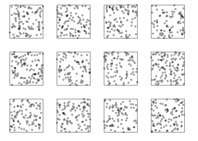
Here are some realisations of the homogeneous Poisson process with intensity 100 (points per unit area):

plot(rpoispp(100, nsim=12), main="", main.panel="")

The inhomogeneous Poisson process with intensity function $\lambda(u)$ is characterised by the following properties:

for any region $B$ , the random number $n(X \cap B)$ of points falling in $B$ follows a Poisson distribution;
for any region $B$ , the expected number of points falling in $B$ is
$E[n(X \cap B)] = \int_B \lambda(u) \, {\rm d}u;$
for any region $B$ , given that $n(X \cap B) = n$ , the $n$ points are independent and identically distributed inside $B$ with probability density $f(u)= \lambda(u)/\Lambda$ , where $\Lambda = \int_B \lambda(u) \, {\rm d}u$ ;
for any disjoint regions $B_1,\ldots, B_m$ , the numbers $n(X \cap B_1), \ldots, n(X \cap B_m)$ of points falling in each region are independent random variables.

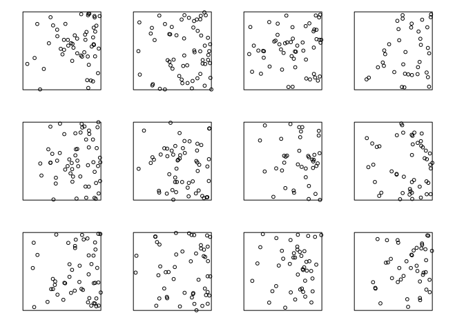
Here are some realisations of the inhomogeneous Poisson process with intensity function $\lambda((x,y)) = 100 x$ :

lam <- function(x,y) { 100 * x}
plot(rpoispp(lam, nsim=12), main="", main.panel="")

Loglinear model for intensity

ppm can fit a Poisson point process model to the point pattern data by maximum likelihood.

A Poisson point process is completely specified by its intensity function. So the procedure for formulating a Poisson model is simply to write a mathematical expression for the intensity function.

In ppm the intensity is assumed to be a loglinear function of the parameters. That is,
$\log\lambda(u) = \beta_1 Z_1(u) + \ldots + \beta_p Z_p(u)$
where $\beta_1, \ldots, \beta_p$ are parameters to be estimated, and $Z_1, \ldots, Z_p$ are spatial covariates.

To fit this model to a point pattern dataset X, we type

ppm(X ~ Z1 + Z2 + .. Zp)

where Z1, Z2, ..., Zp are pixel images or functions.

Important notes:

The model is expressed in terms of the log of the intensity.
The covariates $Z_1(u), \ldots, Z_p(u)$ (called the “canonical covariates”) can be anything; they are not necessarily the same as the original variables that we were given; they could be transformations and combinations of the original variables.

Fit by maximum likelihood

The Poisson process with intensity function $\lambda_\theta(u)$ , controlled by a parameter vector $\theta$ , has log-likelihood
$\log L(\theta) = \sum_{i=1}^n \log \lambda_\theta(x_i) - \int_W \lambda_\theta(u) \, {\rm d} u.$
The value of $\theta$ which maximises $\log L(\theta)$ is taken as the parameter estimate $\hat\theta$ .

From $\hat\theta$ we can compute the fitted intensity $\hat\lambda(u) = \lambda_{\hat\theta}(u)$ and hence we can generate simulated realisations.

Using the likelihood we are able to compute confidence intervals, perform analysis of deviance, conduct hypothesis tests, etc.

Example: Murchison gold data

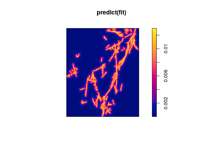
Using the Murchison data from above,

fit <- ppm(X ~ D)

The formula implies that the model is
$\log\lambda(u) = \beta_0 + \beta_1 D(u)$
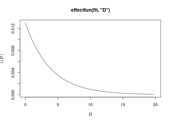
where $D(u)$ is the distance covariate (distance from location $u$ to nearest geological fault) and $\beta_0, \beta_1$ are the regression coefficients. In other words, the model says that the intensity of gold deposits is an exponentially decreasing function of distance from the nearest fault.

The result of ppm is a fitted model object of class "ppm". There are many methods for this class:

fit

## Nonstationary Poisson process
## 
## Log intensity:  ~D
## 
## Fitted trend coefficients:
## (Intercept)           D 
##  -4.3412775  -0.2607664 
## 
##               Estimate       S.E.    CI95.lo    CI95.hi Ztest      Zval
## (Intercept) -4.3412775 0.08556260 -4.5089771 -4.1735779   *** -50.73802
## D           -0.2607664 0.02018789 -0.3003339 -0.2211988   *** -12.91697

coef(fit)

## (Intercept)           D 
##  -4.3412775  -0.2607664

confint(fit)

##                  2.5 %     97.5 %
## (Intercept) -4.5089771 -4.1735779
## D           -0.3003339 -0.2211988

anova(fit, test="Chi")

## Analysis of Deviance Table
## Terms added sequentially (first to last)
## 
##      Df Deviance Npar  Pr(>Chi)    
## NULL                1              
## D     1   590.92    2 < 2.2e-16 ***
## ---
## Signif. codes:  0 '***' 0.001 '**' 0.01 '*' 0.05 '.' 0.1 ' ' 1

plot(predict(fit))

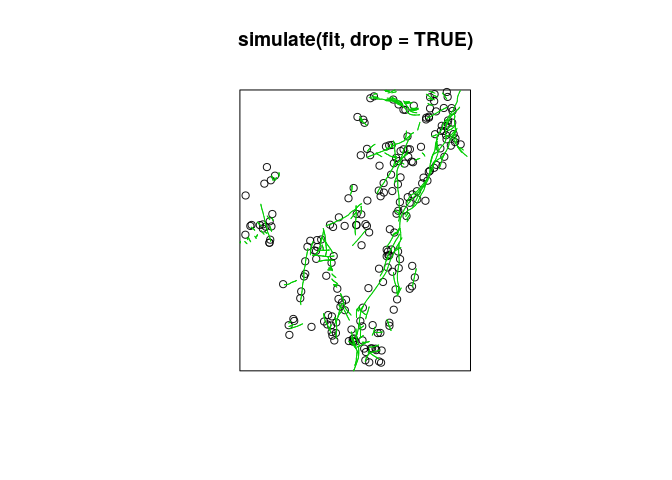
plot(simulate(fit, drop=TRUE))
plot(L, add=TRUE, col=3)

To visualise the intensity of the model as a function of one of the covariates, we can use the command effectfun:

plot(effectfun(fit, "D"), xlim=c(0, 20))

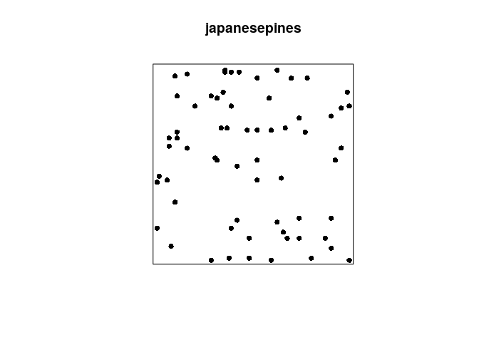
Example: Japanese Pines data

plot(japanesepines, pch=16)

The symbols x, y refer to the Cartesian coordinates, and can be used to model spatial variation in the intensity when no other covariates are available:

Jfit <- ppm(japanesepines ~ x + y)
Jfit

## Nonstationary Poisson process
## 
## Log intensity:  ~x + y
## 
## Fitted trend coefficients:
## (Intercept)           x           y 
##   4.0670790  -0.2349641   0.4296171 
## 
##               Estimate      S.E.    CI95.lo   CI95.hi Ztest       Zval
## (Intercept)  4.0670790 0.3341802  3.4120978 4.7220602   *** 12.1703167
## x           -0.2349641 0.4305456 -1.0788181 0.6088898       -0.5457357
## y            0.4296171 0.4318102 -0.4167154 1.2759495        0.9949211

confint(Jfit)

##                  2.5 %    97.5 %
## (Intercept)  3.4120978 4.7220602
## x           -1.0788181 0.6088898
## y           -0.4167154 1.2759495

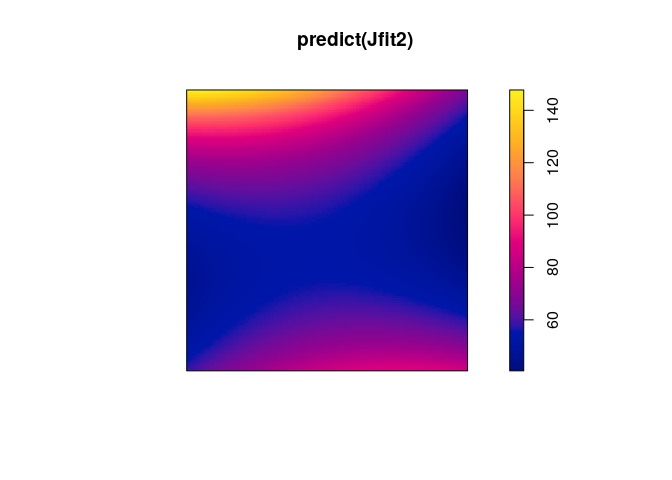
Jfit2 <- ppm(japanesepines ~ polynom(x,y,2))
Jfit2

## Nonstationary Poisson process
## 
## Log intensity:  ~x + y + I(x^2) + I(x * y) + I(y^2)
## 
## Fitted trend coefficients:
## (Intercept)           x           y      I(x^2)    I(x * y)      I(y^2) 
##   4.0645501   1.1436854  -1.5613621  -0.7490094  -1.2009245   2.5061569 
## 
##               Estimate      S.E.    CI95.lo  CI95.hi Ztest       Zval
## (Intercept)  4.0645501 0.6670766  2.7571041 5.371996   ***  6.0930788
## x            1.1436854 1.9589569 -2.6957995 4.983170        0.5838237
## y           -1.5613621 1.8738722 -5.2340841 2.111360       -0.8332277
## I(x^2)      -0.7490094 1.7060242 -4.0927554 2.594737       -0.4390380
## I(x * y)    -1.2009245 1.4268186 -3.9974376 1.595589       -0.8416799
## I(y^2)       2.5061569 1.6013679 -0.6324664 5.644780        1.5650101

plot(predict(Jfit2))

anova(Jfit, Jfit2, test="Chi")

## Analysis of Deviance Table
## 
## Model 1: ~x + y   Poisson
## Model 2: ~x + y + I(x^2) + I(x * y) + I(y^2)      Poisson
##   Npar Df Deviance Pr(>Chi)
## 1    3                     
## 2    6  3   3.3851    0.336

step(Jfit2)

## Start:  AIC=-405.35
## ~x + y + I(x^2) + I(x * y) + I(y^2)
## 
##            Df     AIC
## - I(x^2)    1 -407.15
## - x         1 -407.00
## - y         1 -406.67
## - I(x * y)  1 -406.63
## <none>        -405.35
## - I(y^2)    1 -404.97
## 
## Step:  AIC=-407.15
## ~x + y + I(x * y) + I(y^2)
## 
##            Df     AIC
## - x         1 -408.96
## - I(x * y)  1 -408.47
## - y         1 -408.45
## <none>        -407.15
## - I(y^2)    1 -406.77
## 
## Step:  AIC=-408.96
## ~y + I(x * y) + I(y^2)
## 
##            Df     AIC
## - I(x * y)  1 -410.17
## - y         1 -409.78
## <none>        -408.96
## - I(y^2)    1 -408.48
## 
## Step:  AIC=-410.17
## ~y + I(y^2)
## 
##          Df     AIC
## - y       1 -410.51
## <none>      -410.17
## - I(y^2)  1 -409.66
## 
## Step:  AIC=-410.51
## ~I(y^2)
## 
##          Df     AIC
## - I(y^2)  1 -410.67
## <none>      -410.51
## 
## Step:  AIC=-410.67
## ~1

## Stationary Poisson process
## Intensity: 65
##             Estimate      S.E.  CI95.lo  CI95.hi Ztest     Zval
## log(lambda) 4.174387 0.1240347 3.931284 4.417491   *** 33.65499

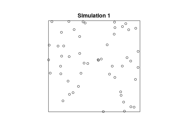
plot(simulate(Jfit2), main = "")

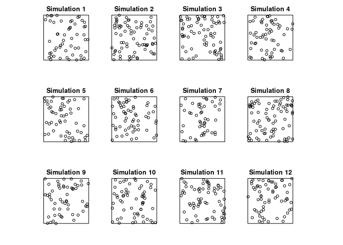
plot(simulate(Jfit2, nsim=12), main = "")

## Generating 12 simulated patterns ...1, 2, 3, 4, 5, 6, 7, 8, 9, 10, 11,  12.

Intensity depending on marks

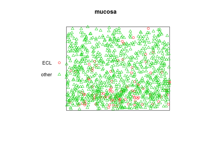
In a multi-type point pattern the points have marks which are categorical values:

mucosa

## Marked planar point pattern: 965 points
## Multitype, with levels = ECL, other 
## window: rectangle = [0, 1] x [0, 0.81] units

plot(mucosa, cols=c(2,3))

We can fit a Poisson model in which the intensity depends on the type of point, using the variable name marks in the model formula.

model0 <- ppm(mucosa ~ marks)
model0

## Stationary multitype Poisson process
## 
## Possible marks: 'ECL' and 'other'
## 
## Log intensity:  ~marks
## 
## Intensities:
##   beta_ECL beta_other 
##   109.8765  1081.4815 
## 
##             Estimate      S.E.  CI95.lo  CI95.hi Ztest     Zval
## (Intercept) 4.699357 0.1059998 4.491602 4.907113   *** 44.33365
## marksother  2.286730 0.1112542 2.068675 2.504784   *** 20.55409

coef(model0)

## (Intercept)  marksother 
##    4.699357    2.286730

plot(predict(model0), equal.ribbon=TRUE)

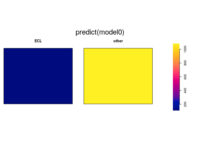
In the formula, the marks variable is a categorical variable. The effect of the model formula mucosa ~ marks is to estimate a different intensity for each level, that is, a different intensity for each type of point. The model formula mucosa ~ marks is equivalent to saying that the intensity of the points of type $i$ is
$\lambda_i(u) = \alpha_i$
for each $i = 1, 2, \ldots$ where $\alpha_1, \alpha_2, \ldots$ are the different constant intensities to be estimated. The actual printed output will depend on the convention for handling “contrasts” in linear models.

The marks variable can be combined with other explanatory variables:

model1 <- ppm(mucosa ~ marks + y)
model1

## Nonstationary multitype Poisson process
## 
## Possible marks: 'ECL' and 'other'
## 
## Log intensity:  ~marks + y
## 
## Fitted trend coefficients:
## (Intercept)  marksother           y 
##    5.131273    2.286730   -1.156055 
## 
##              Estimate      S.E.   CI95.lo    CI95.hi Ztest      Zval
## (Intercept)  5.131273 0.1164479  4.903039  5.3595066   *** 44.064966
## marksother   2.286730 0.1112542  2.068675  2.5047840   *** 20.554089
## y           -1.156055 0.1406821 -1.431787 -0.8803236   *** -8.217504

coef(model1)

## (Intercept)  marksother           y 
##    5.131273    2.286730   -1.156055

plot(predict(model1))

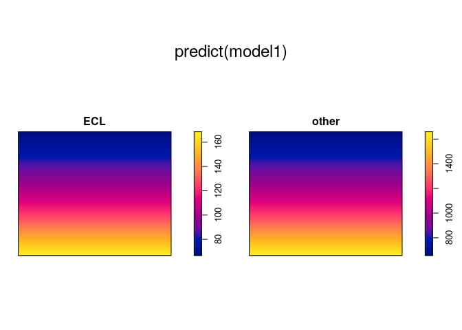
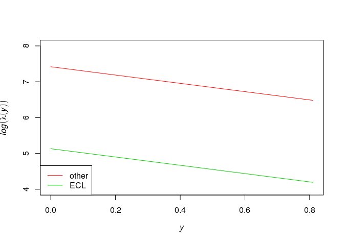
The model formula ~marks + y states that
$\log \lambda_i((x,y)) = \gamma_i + \beta y$
where $\gamma_1, \gamma_2, \ldots$ and $\beta$ are parameters. That is, the dependence on the $y$ coordinate has the same “slope” coefficient $\beta$ for each type of point, but different types of points have different abundance overall.

## This requires spatstat 1.60-1.006 or later
if(packageVersion("spatstat") < "1.60-1.006"){
  message("This version of spatstat cannot produce the relevant type of effect plot.")
} else{
  plot(effectfun(model1, "y", marks="other"),
       log(.y) ~ .x, ylim=c(4,8), col=2, main="")
  plot(effectfun(model1, "y", marks="ECL"),
        add=TRUE, col=3, log(.y) ~ .x)
  legend("bottomleft", lwd=c(1,1), col=c(2,3), legend=c("other", "ECL"))
}

model2 <- ppm(mucosa ~ marks * y)
model2

## Nonstationary multitype Poisson process
## 
## Possible marks: 'ECL' and 'other'
## 
## Log intensity:  ~marks * y
## 
## Fitted trend coefficients:
##  (Intercept)   marksother            y marksother:y 
##     5.884603     1.452251    -3.862202     2.938790 
## 
##               Estimate      S.E.   CI95.lo   CI95.hi Ztest      Zval
## (Intercept)   5.884603 0.1635842  5.563984  6.205222   *** 35.972936
## marksother    1.452251 0.1749458  1.109364  1.795139   ***  8.301149
## y            -3.862202 0.5616953 -4.963104 -2.761299   *** -6.875973
## marksother:y  2.938790 0.5804890  1.801053  4.076528   ***  5.062611

coef(model2)

##  (Intercept)   marksother            y marksother:y 
##     5.884603     1.452251    -3.862202     2.938790

plot(predict(model2))

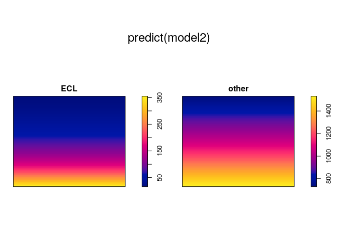
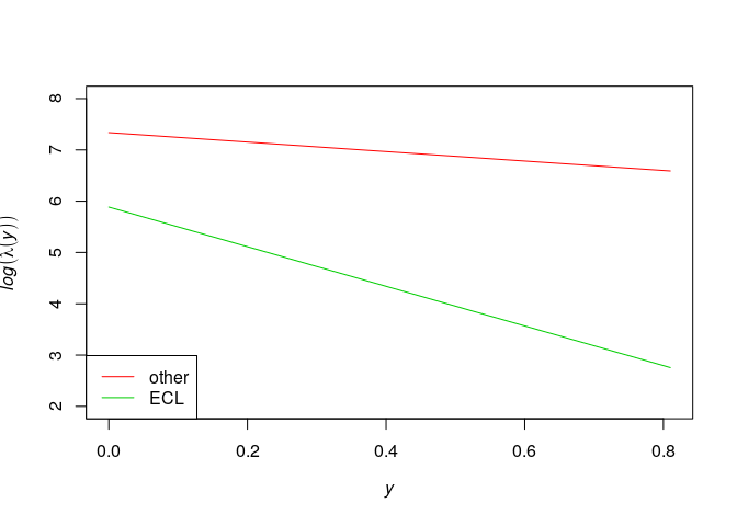
The model formula ~marks * y states that
$\log \lambda_i((x,y)) = \gamma_i + \beta_i y$
where $\gamma_1, \gamma_2, \ldots$ and $\beta_1,\beta_2, \ldots$ are parameters. The intensity may depend on the $y$ coordinate in a completely different way for different types of points.

## This requires spatstat 1.60-1.006 or later
if(packageVersion("spatstat") < "1.60-1.006"){
  message("This version of spatstat cannot produce the relevant type of effect plot.")
} else{
  plot(effectfun(model2, "y", marks="other"),
       log(.y) ~ .x, col=2, ylim=c(2,8), main="")
  plot(effectfun(model2, "y", marks="ECL"),
       add=TRUE, col=3, log(.y) ~ .x)
  legend("bottomleft", lwd=c(1,1), col=c(2,3), legend=c("other", "ECL"))
}

Other examples to discuss:

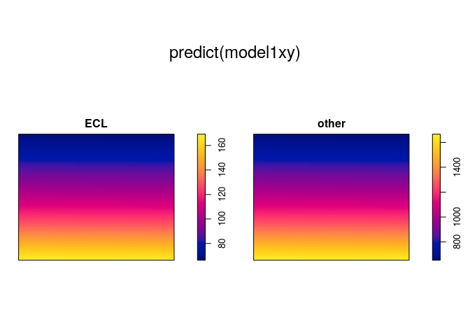
model1xy <- ppm(mucosa ~ marks + x + y)
model1xy

## Nonstationary multitype Poisson process
## 
## Possible marks: 'ECL' and 'other'
## 
## Log intensity:  ~marks + x + y
## 
## Fitted trend coefficients:
##  (Intercept)   marksother            x            y 
##  5.135026706  2.286729721 -0.007512035 -1.156055806 
## 
##                 Estimate      S.E.    CI95.lo    CI95.hi Ztest       Zval
## (Intercept)  5.135026706 0.1290806  4.8820333  5.3880201   *** 39.7815429
## marksother   2.286729721 0.1112542  2.0686754  2.5047840   *** 20.5540892
## x           -0.007512035 0.1115200 -0.2260873  0.2110632       -0.0673604
## y           -1.156055806 0.1406820 -1.4317876 -0.8803241   *** -8.2175076

coef(model1xy)

##  (Intercept)   marksother            x            y 
##  5.135026706  2.286729721 -0.007512035 -1.156055806

plot(predict(model1xy))

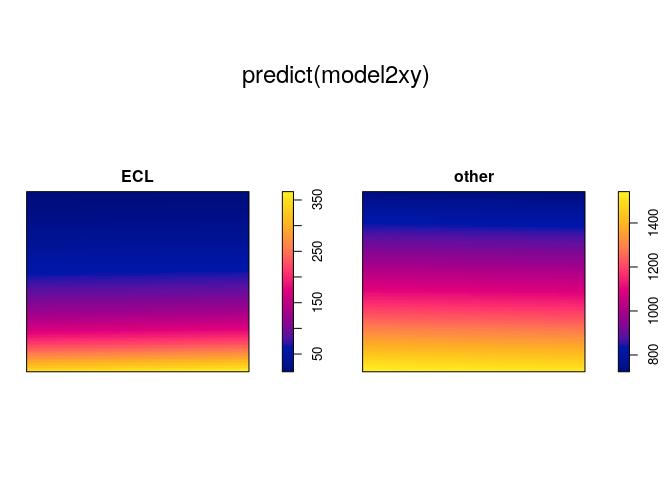
model2xy <- ppm(mucosa ~ marks * (x + y))
model2xy

## Nonstationary multitype Poisson process
## 
## Possible marks: 'ECL' and 'other'
## 
## Log intensity:  ~marks * (x + y)
## 
## Fitted trend coefficients:
##  (Intercept)   marksother            x            y marksother:x 
##   5.85306325   1.49110635   0.06275125  -3.86220183  -0.07739871 
## marksother:y 
##   2.93878953 
## 
##                 Estimate      S.E.    CI95.lo    CI95.hi Ztest       Zval
## (Intercept)   5.85306325 0.2473601  5.3682464  6.3378801   *** 23.6621186
## marksother    1.49110635 0.2616142  0.9783520  2.0038607   ***  5.6996392
## x             0.06275125 0.3672459 -0.6570374  0.7825399        0.1708699
## y            -3.86220183 0.5616962 -4.9631062 -2.7612975   *** -6.8759620
## marksother:x -0.07739871 0.3854477 -0.8328623  0.6780649       -0.2008021
## marksother:y  2.93878953 0.5804899  1.8010502  4.0765289   ***  5.0626022

coef(model2xy)

##  (Intercept)   marksother            x            y marksother:x 
##   5.85306325   1.49110635   0.06275125  -3.86220183  -0.07739871 
## marksother:y 
##   2.93878953

plot(predict(model2xy))

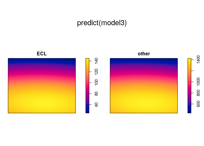
model3 <- ppm(mucosa ~ marks + polynom(x, y, 2))
model3

## Nonstationary multitype Poisson process
## 
## Possible marks: 'ECL' and 'other'
## 
## Log intensity:  ~marks + (x + y + I(x^2) + I(x * y) + I(y^2))
## 
## Fitted trend coefficients:
## (Intercept)  marksother           x           y      I(x^2)    I(x * y) 
##   4.8407551   2.2867297   0.2828123   0.8046386  -0.2449076  -0.1328756 
##      I(y^2) 
##  -2.5066916 
## 
##               Estimate      S.E.    CI95.lo    CI95.hi Ztest       Zval
## (Intercept)  4.8407551 0.1865057  4.4752107  5.2062995   *** 25.9550007
## marksother   2.2867297 0.1112542  2.0686754  2.5047840   *** 20.5540892
## x            0.2828123 0.4840067 -0.6658233  1.2314479        0.5843149
## y            0.8046386 0.6087936 -0.3885748  1.9978521        1.3216937
## I(x^2)      -0.2449076 0.4346487 -1.0968034  0.6069882       -0.5634611
## I(x * y)    -0.1328756 0.5195314 -1.1511385  0.8853873       -0.2557605
## I(y^2)      -2.5066916 0.7025926 -3.8837479 -1.1296354   *** -3.5677739

coef(model3)

## (Intercept)  marksother           x           y      I(x^2)    I(x * y) 
##   4.8407551   2.2867297   0.2828123   0.8046386  -0.2449076  -0.1328756 
##      I(y^2) 
##  -2.5066916

plot(predict(model3))

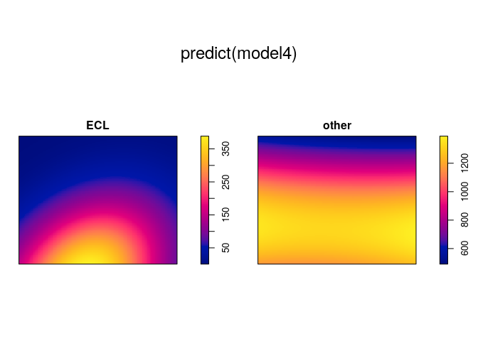
model4 <- ppm(mucosa ~ marks * polynom(x,y,2))
model4

## Nonstationary multitype Poisson process
## 
## Possible marks: 'ECL' and 'other'
## 
## Log intensity:  ~marks * (x + y + I(x^2) + I(x * y) + I(y^2))
## 
## Fitted trend coefficients:
##         (Intercept)          marksother                   x 
##            5.018632            2.040831            4.310737 
##                   y              I(x^2)            I(x * y) 
##           -2.261047           -4.905847            3.086670 
##              I(y^2)        marksother:x        marksother:y 
##           -5.199005           -4.388268            3.579736 
##   marksother:I(x^2) marksother:I(x * y)   marksother:I(y^2) 
##            5.059764           -3.342710            2.439852 
## 
##                      Estimate      S.E.     CI95.lo    CI95.hi Ztest
## (Intercept)          5.018632 0.5006414   4.0373924  5.9998706   ***
## marksother           2.040831 0.5278293   1.0063043  3.0753570   ***
## x                    4.310737 1.7516879   0.8774918  7.7439820     *
## y                   -2.261047 2.2251226  -6.6222072  2.1001133      
## I(x^2)              -4.905847 1.6650184  -8.1692227 -1.6424705    **
## I(x * y)             3.086670 2.6191912  -2.0468503  8.2201905      
## I(y^2)              -5.199005 3.0833891 -11.2423363  0.8443271      
## marksother:x        -4.388268 1.8233568  -7.9619815 -0.8145540     *
## marksother:y         3.579736 2.3165955  -0.9607074  8.1201802      
## marksother:I(x^2)    5.059764 1.7252514   1.6783335  8.4411947    **
## marksother:I(x * y) -3.342710 2.6736718  -8.5830101  1.8975907      
## marksother:I(y^2)    2.439852 3.1699025  -3.7730426  8.6527470      
##                           Zval
## (Intercept)         10.0244036
## marksother           3.8664599
## x                    2.4609047
## y                   -1.0161449
## I(x^2)              -2.9464219
## I(x * y)             1.1784822
## I(y^2)              -1.6861331
## marksother:x        -2.4066971
## marksother:y         1.5452574
## marksother:I(x^2)    2.9327692
## marksother:I(x * y) -1.2502319
## marksother:I(y^2)    0.7696931

coef(model4)

##         (Intercept)          marksother                   x 
##            5.018632            2.040831            4.310737 
##                   y              I(x^2)            I(x * y) 
##           -2.261047           -4.905847            3.086670 
##              I(y^2)        marksother:x        marksother:y 
##           -5.199005           -4.388268            3.579736 
##   marksother:I(x^2) marksother:I(x * y)   marksother:I(y^2) 
##            5.059764           -3.342710            2.439852

plot(predict(model4))

Parametric estimation of spatially-varying probability

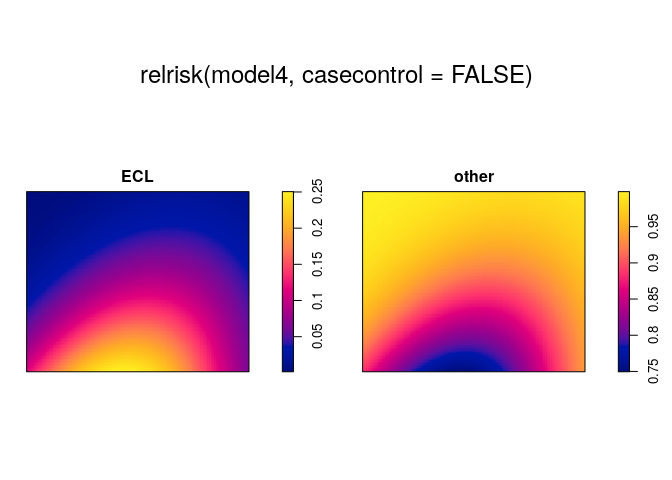
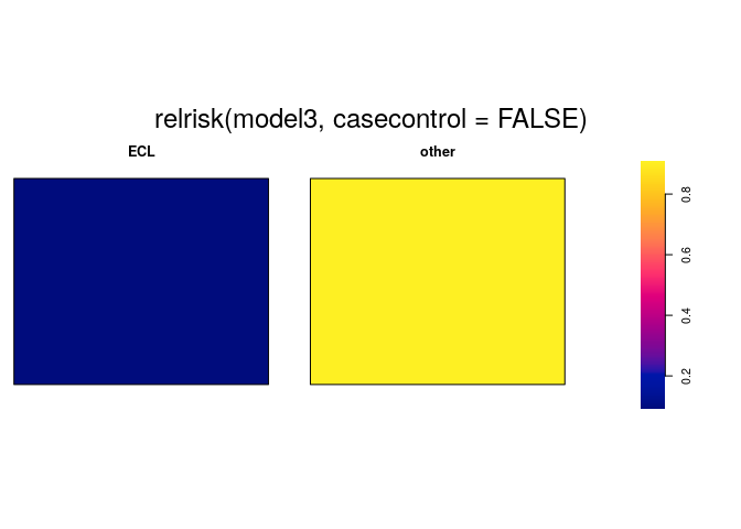
When we have fitted a point process model to a multi-type point pattern, we can compute ratios of the intensities of different types. This is automated in relrisk.ppm:

plot(relrisk(model4, casecontrol=FALSE))

plot(relrisk(model3, casecontrol=FALSE), equal.ribbon=TRUE)

Test for segregation

One way to test for segregation is to compare two models, with the null model stating that there is no segregation:

nullmodel <- ppm(mucosa ~ marks + polynom(x, y, 2))
altmodel <- ppm(mucosa ~ marks * polynom(x, y, 2))
anova(nullmodel, altmodel, test="Chi")

## Analysis of Deviance Table
## 
## Model 1: ~marks + (x + y + I(x^2) + I(x * y) + I(y^2))    Poisson
## Model 2: ~marks * (x + y + I(x^2) + I(x * y) + I(y^2))    Poisson
##   Npar Df Deviance  Pr(>Chi)    
## 1    7                          
## 2   12  5   44.834 1.568e-08 ***
## ---
## Signif. codes:  0 '***' 0.001 '**' 0.01 '*' 0.05 '.' 0.1 ' ' 1