ECAS2019

Notes for session 1

Adrian Baddeley and Ege Rubak July 15, 2019

Introduction

Spatial data= data attributed to spatial locations

Three main types of spatial data:

spatial variable (“field”), eg temperature
regional aggregate data, eg accident counts in each state
spatial point patterns, eg locations of crimes/accidents

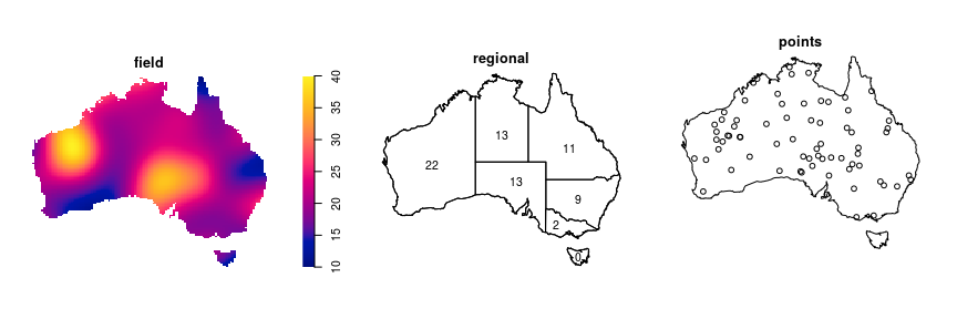
This workshop is about the analysis of spatial point patterns

We will use the spatstat package in R

library(spatstat)

Spatial point pattern terminology

Points

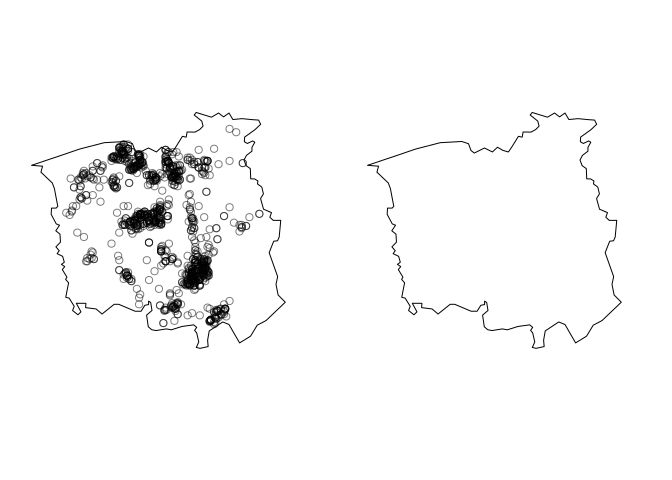
The “points” in a point pattern are the spatial locations where the events or objects were observed. They are specified by spatial coordinates. NOTE: In all that follows and for all functions in spatstat the coordinates are assumed to be projected coordinates in Euclidean space. Do not analyse geographic coordinates (latitude and longitude) directly in spatstat – project them first!

Window

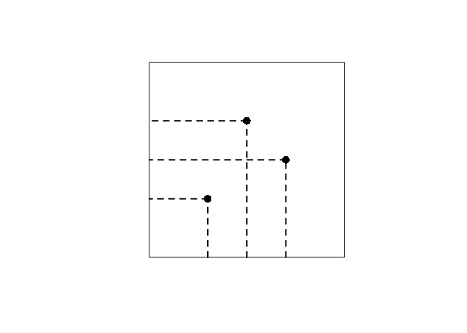
The window $W$ is the spatial region where points were (or could have been) observed.

Covariates

Covariates are explanatory variables (which might “explain” any spatial variation in the abundance of points, for example).

Many covariates take the form of a function $Z(u), \quad u \in W$ defined at every spatial location $u$ .

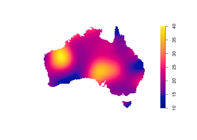
Alternatively, other kinds of spatial data can be treated as explanatory data. Usually we need to translate them into spatial functions for use in analysis.

Marks

Marks are attributes of the individual events or things.

In a spatial point pattern of trees, the trees might be classified into different species, and each tree carries a mark (“label”) indicating which species it belongs to.

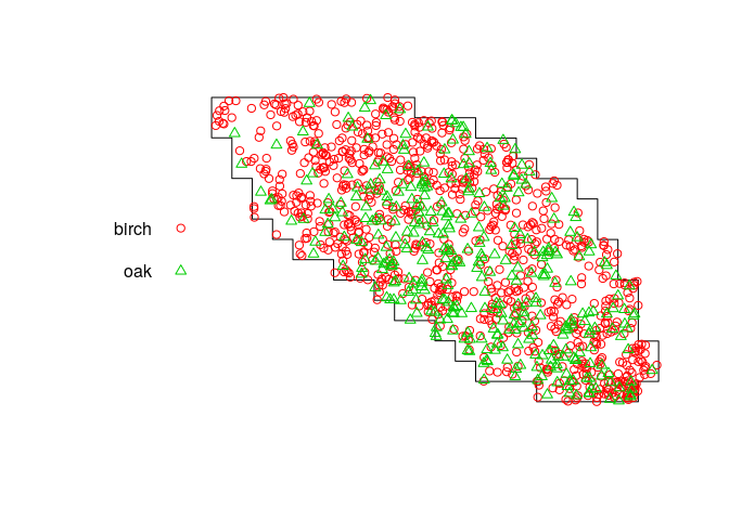
Marks are methodologically different from covariates: marks are part of the “response”, not the “ explanatory variable”

Software and data

Spatstat

library(spatstat)

A point pattern dataset is represented an object belonging to the class "ppp" (planar point pattern). Some datasets are included in the package:

gordon

## Planar point pattern: 99 points
## window: polygonal boundary
## enclosing rectangle: [-26.408475, 26.408475] x [-36.32095, 36.32095] 
## metres

class(gordon)

## [1] "ppp"

plot(gordon)

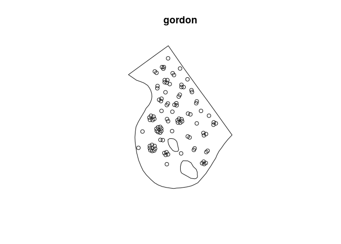
The spatial coordinates of the points can be extracted by as.data.frame:

head(as.data.frame(gordon))

##              x        y
## 1  -6.19217799 29.89951
## 2 -12.95754899 23.24862
## 3 -11.57636899 15.81453
## 4  -0.09553099 24.72807
## 5   0.61446701 16.43510
## 6   0.61446701 15.30598

The window of observation for a point pattern can be extracted by:

W <- Window(gordon)
W

## window: polygonal boundary
## enclosing rectangle: [-26.408475, 26.408475] x [-36.32095, 36.32095] 
## metres

class(W)

## [1] "owin"

This is an object of class "owin" (observation window) representing a spatial region.

If the points also carry marks, the marks can be extracted by marks() or as.data.frame:

hyytiala

## Marked planar point pattern: 168 points
## Multitype, with levels = aspen, birch, pine, rowan 
## window: rectangle = [0, 20] x [0, 20] metres

marks(hyytiala)

##   [1] pine  pine  pine  pine  pine  pine  pine  pine  pine  pine  pine 
##  [12] pine  pine  pine  pine  pine  pine  pine  pine  pine  pine  pine 
##  [23] pine  pine  pine  pine  pine  pine  pine  pine  pine  pine  pine 
##  [34] pine  pine  pine  pine  pine  pine  pine  pine  pine  pine  pine 
##  [45] pine  pine  pine  pine  pine  pine  pine  pine  pine  pine  pine 
##  [56] pine  pine  pine  pine  pine  pine  pine  pine  pine  pine  pine 
##  [67] pine  pine  pine  pine  pine  pine  pine  pine  pine  pine  pine 
##  [78] pine  pine  pine  pine  pine  pine  pine  pine  pine  pine  pine 
##  [89] pine  pine  pine  pine  pine  pine  pine  pine  pine  pine  pine 
## [100] pine  pine  pine  pine  pine  pine  pine  pine  pine  pine  pine 
## [111] pine  pine  pine  pine  pine  pine  pine  pine  pine  pine  pine 
## [122] pine  pine  pine  pine  pine  pine  pine  birch birch birch birch
## [133] birch birch birch birch birch birch birch birch birch birch birch
## [144] birch birch rowan rowan rowan rowan rowan rowan rowan rowan rowan
## [155] rowan rowan rowan rowan rowan rowan rowan rowan rowan rowan rowan
## [166] rowan rowan aspen
## Levels: aspen birch pine rowan

If the marks are a factor (categorical variable) then this specifies a classification of the points into different groups.

The marks could also be numeric:

longleaf

## Marked planar point pattern: 584 points
## marks are numeric, of storage type  'double'
## window: rectangle = [0, 200] x [0, 200] metres

marks(longleaf)

##   [1] 32.9 53.5 68.0 17.7 36.9 51.6 66.4 17.7 21.9 25.7 25.5 28.3 11.2 33.8
##  [15]  2.5  4.2  2.5 31.2 16.4 53.2 67.3 37.8 49.9 46.3 40.5 57.7 58.0 54.9
##  [29] 25.3 18.4 72.0 31.4 55.1 36.0 28.4 24.8 44.1 50.9 47.5 58.0 36.9 65.6
##  [43] 52.9 39.5 42.7 44.4 40.3 53.5 44.2 53.8 38.0 48.3 42.9 40.6 34.5 45.7
##  [57] 51.8 52.0 44.5 35.6 19.2 43.5 33.7 43.3 36.6 46.3 48.3 20.4 40.5 44.0
##  [71] 40.9 51.0 36.5 42.1 15.6 18.5 43.0 28.9 21.3 30.9 42.7 37.6 47.1 44.6
##  [85] 44.3 26.1 25.9 41.4 59.5 26.1 11.4 33.4 35.8 54.4 33.6 35.5  7.4 36.6
##  [99] 19.1 34.9 37.3 16.3 39.1 36.5 25.0 46.8 18.7 23.2 20.4 42.3 38.1 17.9
## [113] 39.7 14.5 33.5 56.0 66.1 26.3 44.8 24.2 39.0 15.1 35.6 21.6 17.2 22.3
## [127] 18.2 55.6 23.3 27.0 50.1 45.5 47.2 37.8 31.9 38.5 23.8 46.3  2.8  3.2
## [141]  5.8  3.5  2.3  3.8  3.2  4.4  3.9  7.8  4.7  4.8 44.1 51.5 51.6 33.3
## [155] 13.3  5.7  3.3 45.9 32.6 11.4  9.1  5.2  4.9 42.0 32.0 32.8 22.0 20.8
## [169]  7.3  3.0  2.2  2.2  2.2 59.4 48.1 51.5 50.3  2.9 19.1 15.1 21.7 42.4
## [183] 40.2 37.4 40.1 39.5 32.5 39.5 35.6 44.1 42.2 39.4 35.5 39.1  9.5 48.4
## [197] 31.9 30.7 15.0 24.5 15.0 22.2 27.5 10.8 26.2 10.2 18.9 44.2 13.8 16.7
## [211] 35.7 12.1 35.4 32.7 30.1 28.4 16.5 12.7  5.5  2.5  3.0  3.2  3.2  4.0
## [225]  3.6  3.8  4.3  3.3  6.3 18.4  5.4  5.4 26.0 22.3 35.2 24.1  6.9 61.0
## [239] 20.6  6.5  2.8  4.8  5.4  4.3  4.0  3.2  2.8  4.9  3.5  2.9  2.4  3.3
## [253]  2.1  2.0  3.9  5.0  2.3  2.2 67.7  2.9  2.4 56.3 39.4 59.5 42.4 63.7
## [267] 66.6 69.3 56.9 23.5  9.1 29.9 14.9 38.7 31.5 27.8 28.5 21.6  2.0  2.6
## [281]  2.3  3.5  3.6  2.6  2.0  2.0  2.7  2.6  2.2  2.7 30.1 16.6 10.4 11.8
## [295] 32.3 33.5 30.5 10.5 13.8 22.8 31.7 10.1 14.5 12.0  2.2  2.3  3.2  3.0
## [309] 50.6  2.6 50.0 52.2  5.2  5.2  6.7 14.0 12.7 59.5 52.0 45.9 18.0 43.5
## [323]  3.3  4.3  7.4 10.1 23.1  8.1  5.7 13.3 12.8 11.6  6.3 20.0  8.9 27.6
## [337]  4.5  9.2  2.3  5.0  4.0 21.8 10.9 14.9 45.0 16.4 43.3 55.6 10.6 45.9
## [351] 45.2 35.5 43.6 44.6 38.8 34.9 17.0 50.4  2.0 33.8 51.1 21.8 46.5  5.6
## [365] 19.6 32.3  3.7  2.7  2.5  2.5  2.4  7.2  7.0 11.8  8.5  9.5  7.0 10.5
## [379]  6.6  6.6  8.8 11.6 48.2 36.2 44.9 43.0 37.5 31.5 39.9 35.5 51.7 36.5
## [393] 40.2  7.8 17.0 36.4 19.6 15.0 28.8 20.1 39.3 37.9 40.6 33.0 35.7 20.6
## [407] 22.0 16.3  5.6  7.4 42.3 43.8 53.0 48.1 41.9 48.0 75.9 40.4 40.9 39.4
## [421] 40.9 17.6 17.8  3.7 19.0 11.2 27.6 14.5 34.4 20.0  2.9  7.3 52.7  8.7
## [435]  3.6  4.6 11.4 11.0 18.7  5.6  2.1  3.3 11.5  2.6  4.4 18.3  7.5 17.2
## [449]  4.6 32.0 56.7 46.0  7.8 54.9 45.5  9.2 13.2 15.3  8.5  2.2 58.8 47.5
## [463] 52.2 56.3 39.8 38.1 38.9  9.7  7.4 22.1 16.9  5.9 10.5  9.5 45.9 11.4
## [477]  7.8 14.4  8.3 30.6 44.4 38.7 41.5 34.5 31.8 39.7 23.3 37.7 43.0 39.2
## [491] 40.4 36.7 48.4 27.9 46.4 38.5 39.4 50.0 51.6 38.7 39.6 29.1 44.0 50.9
## [505] 50.8 43.0 44.5 29.8 44.3 51.2 37.7 36.8 33.6 47.9 32.0 40.3 42.5 59.7
## [519] 44.2 30.9 39.5 48.7 32.8 47.2 42.1 43.8 30.5 28.3 10.4 15.0  7.4 15.3
## [533] 17.5  5.0 12.2  9.0  2.4 13.7 13.1 12.8 27.0  2.6  4.9 35.0 23.7 42.9
## [547] 14.2  3.3 28.4 10.0  6.4 22.0  4.3 10.0  9.2  3.7 66.7 68.0 23.1  5.7
## [561] 11.7 40.4 43.3 60.2 55.5 54.1 22.3 21.4 55.7 51.4 23.9  5.2  7.6 27.8
## [575] 49.6 51.0 50.7 43.4 55.6  4.3  2.5 23.5  8.0 11.7

The marks could be multivariate:

finpines

## Marked planar point pattern: 126 points
## Mark variables: diameter, height 
## window: rectangle = [-5, 5] x [-8, 2] metres

head(marks(finpines))

##   diameter height
## 1        1    1.7
## 2        1    1.7
## 3        1    1.6
## 4        5    4.1
## 5        3    3.1
## 6        4    4.3

Other kinds of spatial objects in spatstat include:

pixel images: class "im"
spatial patterns of line segments: class "psp"
spatial tessellations: class "tess"

Wrangling data

In this workshop, we will use datasets which are already installed in spatstat, because time is short.

In practice, you would need to import your own data into R.

Data can be provided in many different file formats

text file, CSV file
shapefile
netcdf file

The spatstat package does not support reading and writing of files in different formats. This would be poor software design.

Instead, if you need to read files in a particular format, we recommend that you find an appropriate R package which is designed to read and write that specific file format. Once the data have been read into R, then you can use another R package to convert the data into objects recognised by spatstat.

It is often enough to use the functions read.table and read.csv in the base R system which will read simple text files containing columns of data and store them in R as a data.frame.

For full details please read the free copy of Chapter 3 of our book